I am a self-taught amateur on remote sensing, but it tickled my pride when a friend at NASA asked me, if I could tell a friend of his at NOAA on how I got my hands on data to produce maps of radar backscatter to describe how the sea ice near Thule Air Base, Greenland changes in time and space.
Wolstenholme Fjord, Greenland Feb.-5, 2017 from Sentinel-1 radar. The data are at 20-m resolution
In about 4 weeks from today I will be working along a line near the red dots A, B, and C which are tentative locations to place ocean sensors below the sea ice after drilling through it with ice fishing gear. The colored line is the bottom depth as it was measured by the USCG Healy in 2003 when I was in Thule for the first time. Faint bottom contours are shown in gray.
I discovered the 20-m Sentinel-1 SAR-C data only 3 weeks ago. They are accessible to me (after making an account) via
where one also finds wonderful instructional videos on how to work the software.
The data file(s) for a typical scene are usually ~800 MB, however, for processing I use the free SNAP software (provided by European Space Agency) via a sequence of steps that result in a geotiff file of about 7 MB.
Screenshot of SNAP software and processing with [1] input and [2] output of the Feb.-5, 2017 data from Wolstenholme Fjord.
This .tiff file I then read with Fortran codes to tailor my own (quantitative or analyses) purposes.
Start of Fortran code to covert the SNAP output geotiff file into an ascii file with latitude, longitude, and backscatter as columns. The code has 143lines plus 80 lines of comment.
The final mapping is done with GMT – General Mapping Tools which I use for almost all my scientific graphing, mapping, and publications.
Please note that I am neither a remote sensing nor a sea-ice expert, but consider myself an observational physical oceanographer who loves his Unix on a MacBook Pro.
Working the Night shift aboard CCGS Henry Larsen in the CTD van in Aug.-2012. [Photo Credit: Renske Gelderloos]
If only my next problem, working in polar bear country with guns for protection, had as easy a solution.
Polar bear as seen in Kennedy Channel on Aug.-12, 2012. [Photo Credit: Kirk McNeil, Labrador from aboard the Canadian Coast Guard Ship Henry Larsen]
Greenland hunters, seals, and polar bears all need sea ice atop a frozen ocean to eat, breath, or live. The sea ice around northern Greenland changes rapidly by becoming thinner, more mobile, and less predictable as a result of warming ocean and air temperatures. I will need to be on the sea ice to the north and west of Thule Air Base in March and April about 6 weeks from to conduct several connected science experiments. The ice should be “land fast,” that is, it should be a solid, not moving plate of ice. The work is funded by the National Science Foundation who asked me to prepare a sea ice safety plan to keep the risk to people working with me to a minimum. In a science plan I included this satellite image of what the ice and land looked like in march of 2016:
Optical satellite image of Wolstenholme Fjord, Greenland on March-21, 2016 with Thule Air Base in bottom right. Darker areas show thin ice.
This LandSat image captures the reflection of sun light during a cloud-free day at ~15 m pixel size. No such imagery exists for 2017 yet, because the sun does not set until late February with this US satellite overhead. The European Space Agency (ESA), however, flies a radar on its Sentinel satellite. This radar sends out its own radio waves that are then reflected back to its antenna. The radar sees not only during the polar night, it can also see through clouds. And ESA provides these data almost instantaneous to anyone who wants it and knows how to deal with large data files. If you think your 8 mega pixels are sharp, these images are closer to 800 mega pixels. Here are three such images from January 3, 24, and 28 (yesterday):
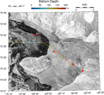
Wolstenholme Fjord, Greenland Jan.-03, 2017 from Sentinel-1 radar.
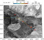
Wolstenholme Fjord, Greenland Jan.-24, 2017 from Sentinel-1 radar.
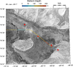
Wolstenholme Fjord, Greenland Jan.-28, 2017 from Sentinel-1 radar.
The lighter white tones indicate that lots of radar signals return to the satellite. The many tiny white specks to the south of the Manson Islands are grounded icebergs. The different shades of gray indicate different types of ice and snow. The Jan.-24 and Jan.-28 images show a clear boundary near longitude of -70 degrees to the north of the island (Saunders Island) that separates land-fast ice to the east from thinner and mobile ice in Baffin Bay to the west.
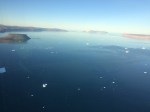
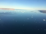
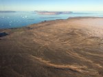
Wolstenholme Fjord on Aug.-27, 2016. The view to the west with Mount Dundas on the left (south) and southern part of Saunders Island on the right (north).
Wolstenholme Fjord on Aug.-27, 2016. The view to the west with the northern part of Saunders Island on the left (south) and smaller Manson Islands on the right (north) next to then northern shore of the fjord.
Wolstenholme Fjord on Aug.-27, 2016. The view to the south-west with Manson Islands in the foreground and Saunders Island in the background
I plan to work from Thule Air Base (red dot bottom right) out along points C, B, towards A. The color of line near these points is a section where I have very accurate bottom depth from a 2003 US Coast Guard Icebreaker that was dropping off scientists at Thule on August 15, 2003. I was then one of the scientist dropped off after a 3 week excursion into Nares Strait and Petermann Fjord. Along this section I hope to test and deploy and under-water acoustic network that can send data via whispers from C to A via B. First, however, we will need to know how sound moves along this track and before that, for my ice safety plan, I will need to know how thick or thin the ice is. The imagery does not tell me ice thickness.
Flying to Thule Greenland with US Air force Air Mobility Command delivering cargo and people.
Arriving in Thule on Mar.-8, we will first need to measure ice thickness along this A-B-C section with a sharp ice-cutting Kovacs drill and a tape measure. The US National Snow and Ice Data Center (NSIDC) distributes a “Handbook for community-based sea ice monitoring” that we will follow closely. This first ice survey will also give us a feel and visual on how the radar satellite imagery displays a range of ice and snow surfaces. One of my PhD students, Pat Ryan, will process and send us the ESA Sentinel-1 radar data while a small University of Delaware and Woods Hole Oceanographic Institution group will work on the ice in early April.
The mental preparation for this scientific travel to Thule and the sea ice beyond gives me the freedom and pleasure to explore new data such as Sentinel-1 imagery and perspectives on tremendous local traditional knowledge of the Inugguit who have lived with the sea ice for perhaps 4000 years. The town of Qaanaaq is 45 minutes by helicopter to the north of Thule Air Base (TAB) at Pituffik. The town was established in 1953 when local populations living in the TAB area were forcibly removed. Despite these challenges the displaced people have prospered throughout the Cold War, but a less predictable and rapidly changing sea ice poses a severe threat to the community whose culture, health, and livelihood still depends on hunting and traveling on sea ice. Stephen Leonard is an anthropological linguist at the University of Cambridge who lived in Qaanaaq for a year in 2010/11 when he made this video:
P.S.: If possible, I would very much like to work with a local person who knows sea ice and wild life that we would need protection from. Danish contacts are reaching out on my behalf to people they know in Siorapaluk, Qaanaaq, and Savissivik.
I am going to sea next week boarding the R/V Sikuliaq in Nome, Alaska to sail for 3 days north into the Arctic Ocean. When we arrive in our study area after all this traveling, then we have perhaps 18 days to deploy 20 ocean moorings. I worry that storms and ice will make our lives at sea miserable. So what does a good data scientist do to prepare him or herself? S/he dives into data:
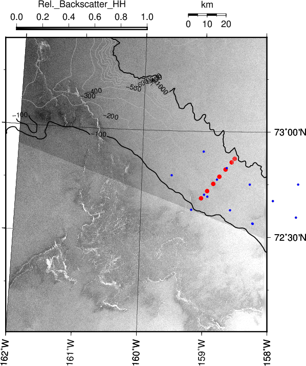
Map northern Chukchi Sea with mooring locations (red and blue symbols), contours of bottom topography, and radar backscatter from space. Slightly darker shades especially in the bottom segment are interpreted as sea ice. The offset in grey scale between top and bottom is caused by me using different numbers for two different data segments to bring the data into a range that varies between 0 and 1.
The image above is my first attempt to determine, if our planned mooring deployment locations are free of sea ice or not. The darker tones of gray are sea ice with the white spots probably thicker or piled-up ridges of rougher sea ice. The speckled gray surface to the north is probably caused by surface waves and other “noise” that are pretty random. There is a data point ever 40 meters in this image. It also helps to compare these very high-resolution ice data with products that the US National Ice Center (NIC) and the National Weather Service provide:
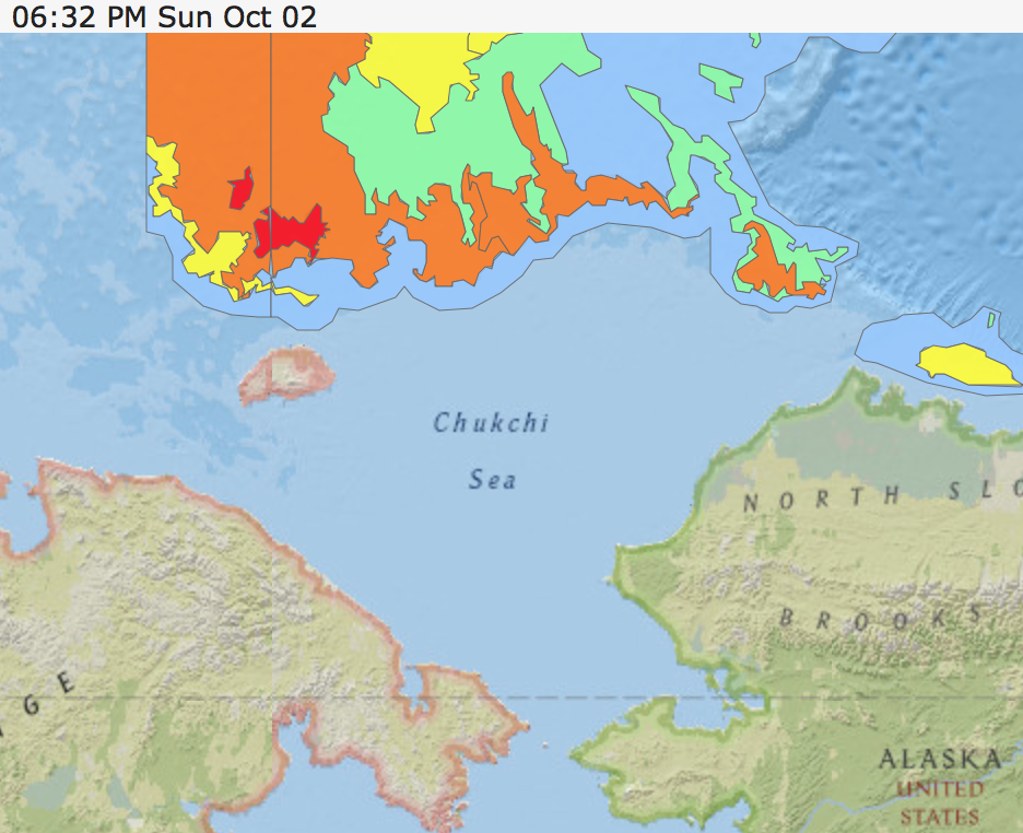
The above is a wonderful map for general orientation, but it is not good or detailed enough to navigate a ship through the ice. The two maps agree, however, my patch of ice to the south of the moorings are represented as the orange/green patch on the top right (north-east). The orange means that 70-80% of the area is covered by ice and this ice is thicker than 1.2 meters and thus too thick for our ship to break through, but there are always pathways through ice and those can be found with the 40-m resolution maps.
In summary, on Sept.-29, 2016 all our moorings are in open water, but this can change, if the wind moves this math northward. So we are also watching the winds and here I like the analyses of Government Canada
Surface weather analysis from Government Canada for Oct.-2, 2016. The map of surface pressure is centered on the north pole with Alaska at the bottom, Europe on the top, Greenland on the right, and Siberia on the left.
It shows a very low pressure center over Siberia to the south-west and a high pressure center over Arctic Canada to our north-east. This implies a strong wind to the north in our study area. So the ice edge will move north into our study area. If the High moves westward, we would be golden, but the general circulation at these latitudes are from west to east, that is, the Low over Siberia will win and move eastward strengthening the northward flow. That’s the bad news for us, but we still have almost 2 weeks before we should be in the area to start placing our fancy ocean moorings carefully into the water below the ice.
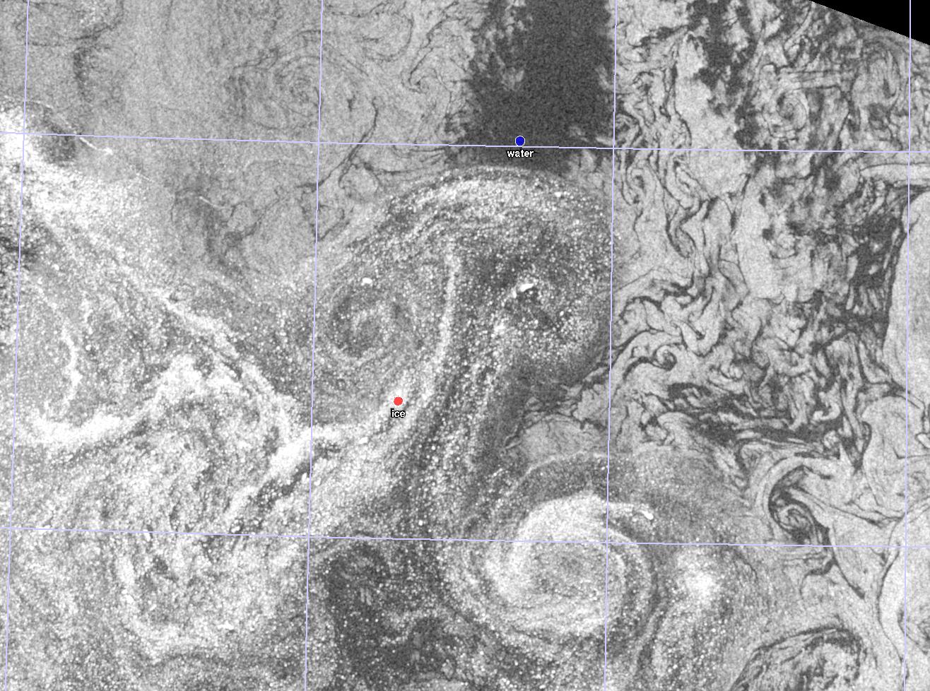
While this “operational” stuff motivated me to dive into the satellite radar data that can “see” through clouds and fog, I am most excited about the discovery that the radar data from the European Space Agency are easy to use with a little clever ingenuity and a powerful laptop (2.5 MHz Mac PowerBook). For example, this hidden gems appeared in the Chukchi Sea a few days earlier:
Close-up of the ice edge in the northern Chukchi Sea on Sept.-23, 2016. The mushroom cloud traced by sea ice and associated eddies are about 10-20 km across.
It is a piece of art, nature’s way to paint the surface of the earth only to destroy this painting the next minute or hour or day to make it all anew. It reminds me of the sand-paintings of some Native American tribes in the South-West of the USA that are washed away the moment they are finished. Here the art is in the painting, just as the pudding is in the eating, and the science is the thinking.
The Manhattan-sized ice island that last year broke free of Petermann Gletscher in North Greenland plowed into the bottom and broke apart. Force equals mass times acceleration. When 18 giga tons (mass) of moving ice crashes into the ocean’s bottom 200 meters below the surface (acceleration), then something gotta give. And give it did, Continue reading →


![Screenshot of SNAP software and processing with [1] input and [2] output of the Feb.-5, 2017 data from Wolstenholme Fjord.](https://icyseas.org/wp-content/uploads/2017/02/screen-shot-2017-02-07-at-5-06-35-pm.png?w=500&h=318)

![Working the Night shift aboard CCGS Henry Larsen in the CTD van in Aug.-2012. [Photo Credit: Renske Gelderloos]](https://icyseas.org/wp-content/uploads/2014/09/aug_8_ctd_andreas_01.jpg?w=500&h=375)
![Polar bear as seen in Kennedy Channel on Aug.-12, 2012. [Photo Credit: Kirk McNeil, Labrador from aboard the Canadian Coast Guard Ship Henry Larsen]](https://icyseas.org/wp-content/uploads/2012/08/polarbear-kirkmcneil_0418.jpg?w=500&h=281)


