Tag Archives: ice

How big is Greenland?

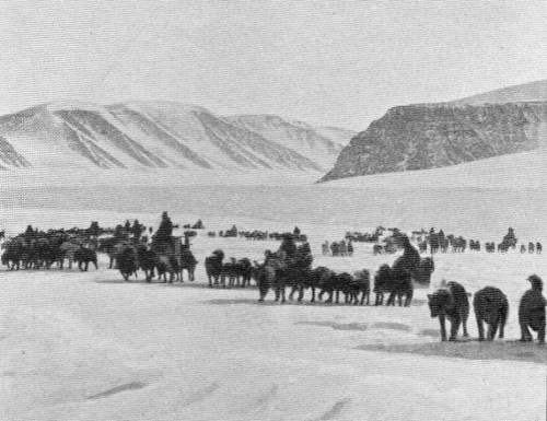
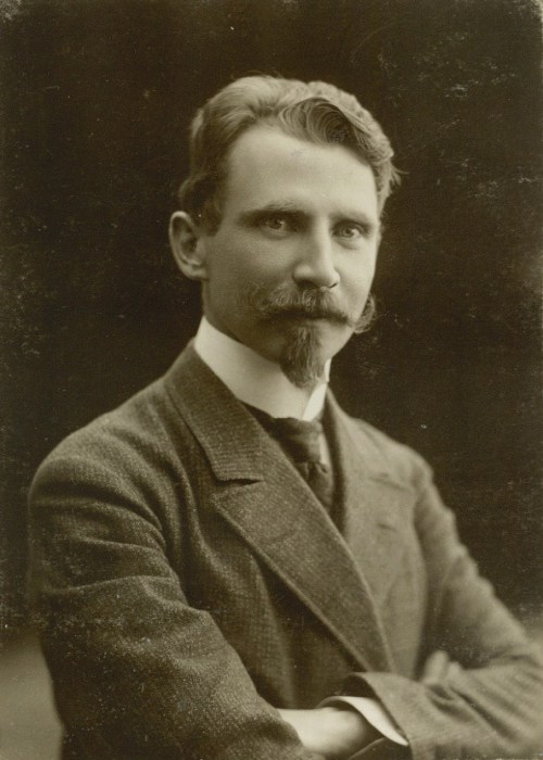
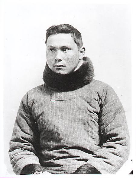
Maps of Greenland were sketched with broken bones, frozen limbs, and starved bodies of men and dogs alike. On April 10, 1912 four men and 53 sled dogs crossed North Greenland from a small Inuit settlement on the West Coast where today the US Air Force maintains Thule Air Base. In 1912 Knud Rassmussen, Peter Freuchen, Uvidloriaq, and Inukitsoq searched for two explorers lost somewhere on Greenland’s East Coast 1200 km (760 miles) away. They returned 5 months later with 8 dogs without finding Einar Mikkelsen or Iver Iversen. These two arrived in North-East Greenland to find diaries, maps, and photos of three earlier explorers who had starved to death in the fall of 1908. Mikkelsen and Iverson found the records, but struggled to survive the winters of 1910/11 and 1911/12 alone stranded before a passing ship found them. I ordered their 1913 Expedition Report yesterday.

Dog sled teams drive across Greenland’s Inland ice in April 1912 from Clemens Markham’s Glacier in the west to Denmark Fjord in the east. All 4 explorers returned, but only 8 dogs did.
Map of Greenland as included in the Report of the First Thule Expedition 1912 by Knud Rasmussen.

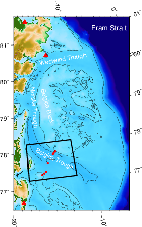
I worked along these coasts in 2014, 2015, 2016, 2017, and 2018 on German research vessels, Swedish icebreakers, Greenland Air helicopters, and American snowmobiles. We explored the oceans below ice and glaciers with digital sensors but without hunger, cold, or lack of comfort. I feel that I know these coasts well, read what others have written and suffered. I make my own maps, too, to reveal patterns of oceans, ice, and glaciers that change in space and time. And yet, I am often lost by distances and areas. I do not know how big Greenland is.

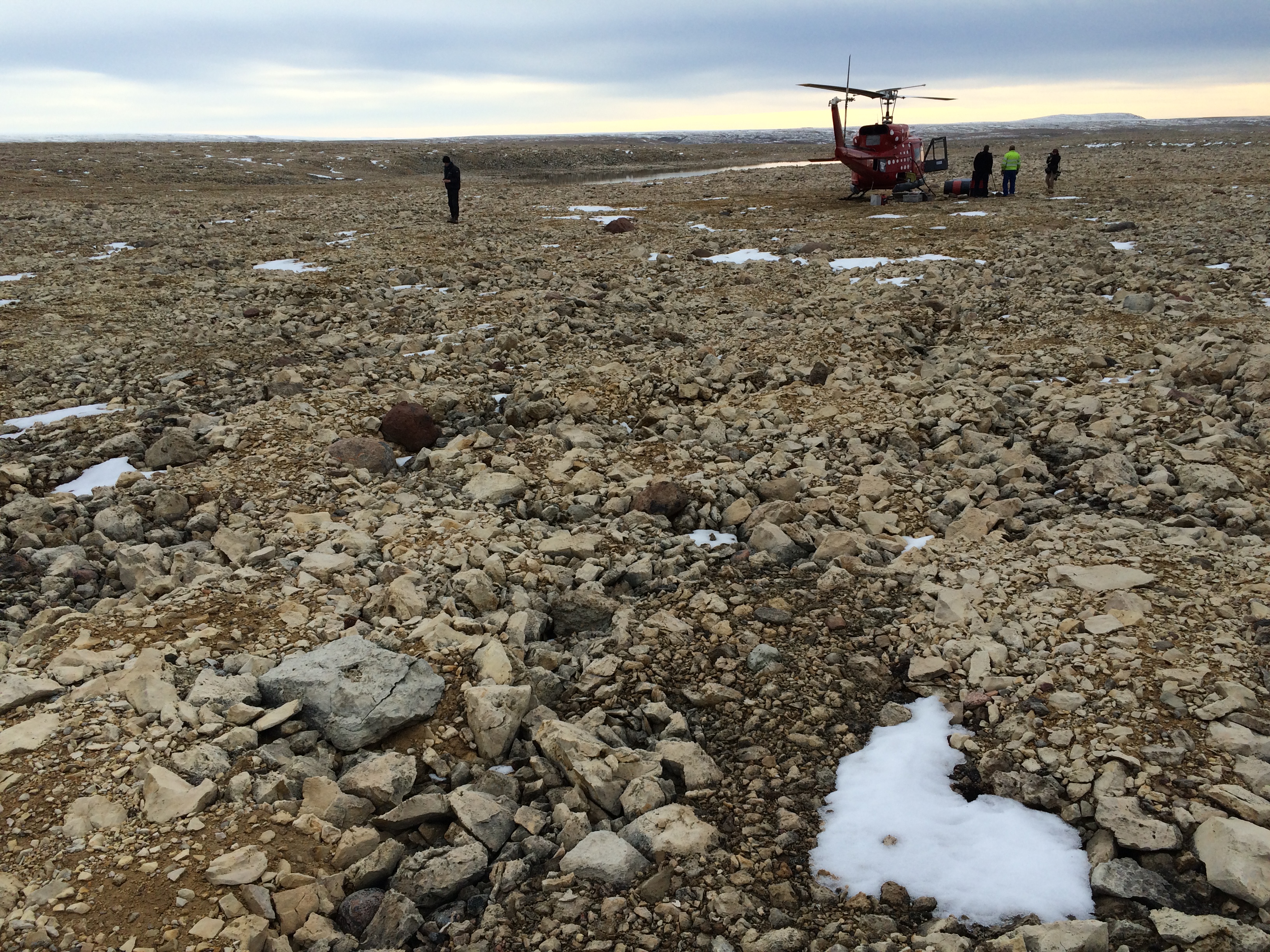
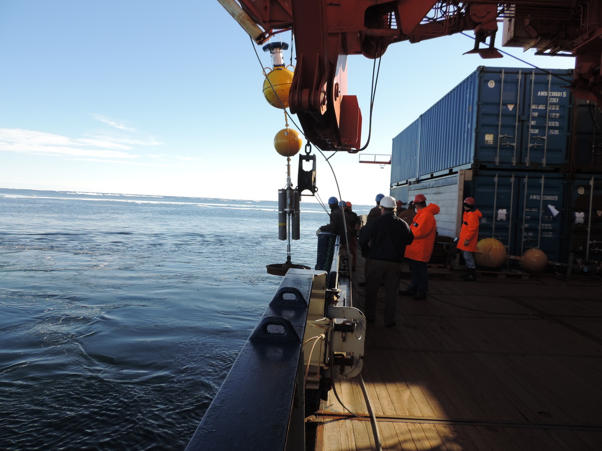
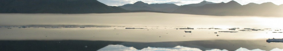
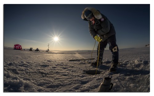
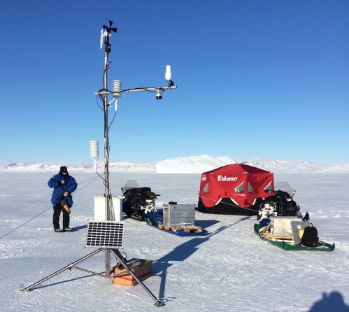
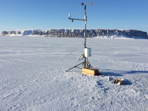
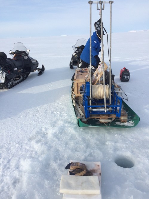
Clockwise from top left: Ocean observatory on sea ice off Thule Air Base (Apr.-2017); refuelling helicopter in transit to ocean observatory on Petermann Gletscher (Aug.-2016); Swedish icebreaker in Baffin Bay (Aug.-2015); and deployment of University of Delaware ocean moorings from Germany’s R/V Polarstern off North-East Greenland at 77 N latitude (Jun.-2014).

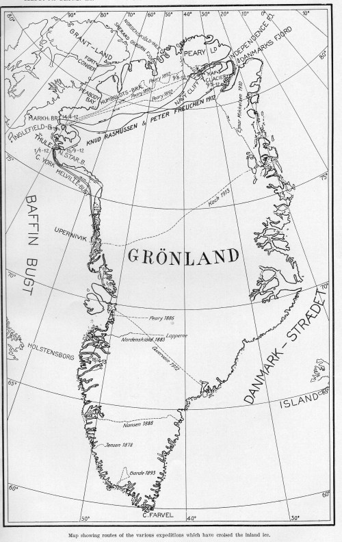
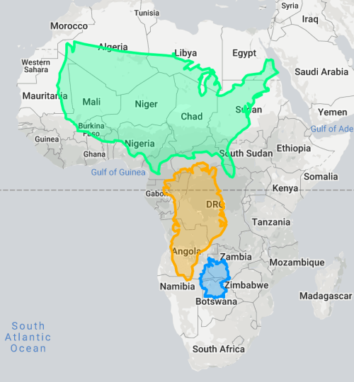
At home I know distances that I walk, bicycle, or drive as part of my daily routine. I know areas where I live from weather and google maps, weekend strolls, and where family and friends live. Once we travel in unfamiliar lands, however, we are lost. Americans rarely know how small most European countries are while Europeans rarely know how far the Americas stretch from Pacific to Atlantic Oceans. Nobody knows the size of Greenland or Africa. On World Atlases Greenland appears as large as Africa, but this is false. Just look at this map:

The size of Africa on the same scale as the USA (green), Greenland (orange), and Germany (blue). Germany is about the same size as Botswana while Greenland is a tad larger than Kongo and the USA is about as big as the Sahara.

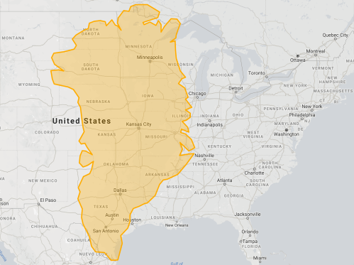
Thus North Greenland’s explorers walked distances similar to walking across Texas, Mississippi, and Florida (and back) or distances similar to walking Germany from its North Sea to the Alps (and back) or distances similar to walking across Kenya (and back). Making these maps, I found the tool at https://thetruesize.com These playful maps compare Greenland’s size by placing its shape onto North-America, Europe, and Asia:

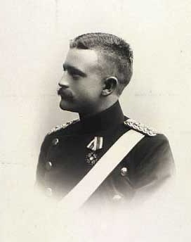
Three explorers starved and froze to death November 1907 because they underestimated their walking area. Their shoes wore thin and they walked barefoot. Daylight disappeared and was replaced by polar night. Food vanished with no game to hunt. Jorgen Bronland, Niels Hoeg Hagen, and Ludvig Mylius-Erichsen were 29, 30, and 35 years young when they died mapping Greenland. I sailed the ice-covered coastal ocean. I was helped by maps they made walking.

Northern Winds and Currents off North-East Greenland

I spent 6 weeks aboard the German research icebreaker R/V Polarstern last year leaving Tromso in Norway in early September and returned to Bremerhaven, Germany in October. We successfully recovered ocean sensors that we had deployed more than 3 years before. It felt good to see old friends, mates, and sensors back on the wooden deck. Many stories, some mysterious, some sad, some funny and happy could be told, but today I am working on some of the data as I reminisce.

The location is North-East Greenland where Fram Strait connects the Arctic Ocean to the north with the Atlantic Ocean in the south. We worked mostly on the shallow continental shelf areas where water depths vary between 50 and 500 meters. The map shows these areas in light bluish tones where the line shows the 100 and 300 meter water depth. Fram Strait is much deeper, more than 2000 meters in places. I am interested how the warm Atlantic water from Fram Strait moves towards the cold glaciers that dot the coastline of Greenland in the west.

Map of study area with 2014-16 mooring array in box near 78 N across Belgica Trough. Red triangles place weather data from Station Nord (81.2 N), Henrik Kr\o yer Holme (80.5 N), and Danmarkhaven (76.9 N). Black box indicates area of mooring locations.

There is also ice, lots of sea icebergs, and ice islands that we had to navigate. None of it did any harm to our gear that we moored for 1-3 years on the ocean floor that can and often is scoured by 100 to 400 meter thick ice from glaciers, however, 2-3 meter thick sea ice prevented us to reach three mooring locations this year and our sensors are still, we hope, on the ocean floor collecting data.

Ahhh, data, here we come. Lets start with the weather at this very lonely place called Henrik Krøyer Holme. The Danish Meteorological Institute (DMI) maintains an automated weather station that, it seems, Dr. Ruth Mottram visited and blogged about in 2014 just before we deployed our moorings from Polarstern back in 2014:

Weather station on Henrik Kroeyer Holme [Credit: Dr. Ruth Mottram, DMI]

It was a little tricky to find the hourly data and it took me more than a day to process and graph it to suit my own purposes, but here it is

Winds (A) and air temperature (B) from an automated weather station at Henrik Kroeyer Holme from 1 June, 2014 through 31 August, 2016. Missing values are indicated as red symbols in (A).

The air temperatures on this island are much warmer than on land to the west, but it still drops to -30 C during a long winter, but the end of July it reaches +5 C. The winds in summer (JJA for June, July, and August) are weak and variable, but they are often ferociously strong in winter (DJF for December, January, February) when they reach almost 30 meters per second (60 knots). The strong winter winds are always from the north moving cold Arctic air to the south. The length of each stick along the time line relates the strength of the winds, that is, long stick indicates much wind. The orientation of each stick indicates the direction that the wind blows, that is, a stick vertical down is a wind from north to south. I use the same type of stick plot for ocean currents. How do these look for the same period?

Ocean current vectors at four selected depths near the eastern wall of Belgica Trough. Note the bottom-intensified flow from south to north. A Lanczos low-pass filter removes variability at time scales smaller than 5 days to emphasize mean and low-frequency variability.

Ocean currents and winds have nothing in common. While the winds are from north to south, the ocean currents are usually in the opposite direction. This becomes particular clear as we compare surface currents at 39 meters below the sea surface with bottom currents 175 or even 255 meters below the surface. They are much stronger and steadier at depth than at the surface. How can this be?

Image of study area on 15 June 2014 with locations (blue symbols) where we deployed moorings a few days before this satellite image was taken by MODIS Terra. The 100-m isobath is shown in red.

Well, recall that there is ice and for much of the year this sea ice is not moving, but is stuck to land and islands. This immobile winter ice protects the ocean below from a direct influence of the local winds. Yet, what is driving such strong flows under the ice? We need to know, because it is these strong currents at 200 to 300 meter depth that move the heat of warm and salty Atlantic waters towards coastal glaciers where they add to the melting of Greenland. This is what I am thinking about now as I am trying to write-up for my German friends and colleagues what we did together the last 3 years.

Oh yes, and we did reach the massive terminus of 79 North Glacier (Nioghalvfjerdsfjorden) that features the largest remaining floating ice shelf in Greenland:

We recovered ocean moorings from this location also, but this is yet another story that is probably best told by scientists at the Alfred-Wegener-Institute who spent much time and treasures to put ship, people, and science on one ship. I am grateful for their support and companionship at sea and hopefully all of next year in Bremerhaven, Germany.

Only in Thule Greenland

… do you find a machinist working metal to take photos while I do oceanography the old-fashioned way by pulling up 100 meters of kevlar line to recover an ocean probe.

Wolstenholme Fjord March-26, 2017. [Photo by Mogens Werth Christensen]

The data were subsequently used by ocean acousticians to test speed of sound propagation as part of an NSF project on testing an underwater communication system to move data from A to B via C or D. The automated weather station reports ocean temperature and saltiness as well at

http://ows.udel.edu/ice

Web-site is low-bandwidth to be used operationally by Air Force personnel in Greenland and local communities where internet access and speeds are severely limited.

Greenland Oceanography by Sled and Snowmobile

Wind chill matters in Greenland because one must see and breath. This implies exposed skin that will hurt and sting at first. Ignoring this sting for a few minutes, I notice that the pain goes away, because the flesh has frozen which kills nerves and skin tissue. The problem becomes worse as one drives by snowmobile to work on the sea ice which I do these days almost every day.

Navigating on the sea ice by identifying ice bergs with LandSat imagery. The imagery also shows polynyas and thin ice in the area. [Photo Credit: Sonny Jacobsen]

Mar.-22, 2017 LandSat image of study area with Thule Air Base near bottom right, Saunders Island in the center. Large red dots are stations A, B, and C with Camp-B containing weather station, shelter, and first ocean mooring. My PhD student Pat Ryan prepared this at the University of Delaware.

My companion on the ice is Sonny Jacobsen who knows and reads the land, ice, and everything living on and below it. He teaches me how to drive the snowmobile, how to watch for tracks in the snow, how to pack a sled, and demonstrates ingenuity to apply tools and materials on-hand to fix a problem good enough to get home and devise a new and better way to get a challenging task done. Here he is designing and rigging what is to become our “Research Sled” R/S Peter Freuchen, but I am a little ahead of my story:

Sonny Jacobsen on Mar.-27, 2017 on Thule Air Base building a self-contained sled for ocean profiling.

First we set up a shelter in the center of what will hopefully soon become an array of ocean sensors and acoustic modems to move data wirelessly through the water from point A in the north-west via point B to point C. Point C will become the pier at Thule Air Base while the tent is at B that I call Camp-B:

Ice Fishing shelter to the north-east of Saunders Island seen to the left in the background.

Next, we set up an automated weather station (AWS) next to this site, because winds and temperatures on land next to hills, glaciers, and ice sheets are not always the same 10 or 20 km offshore in the fjord. It is a risk-mitigating safety factor to know the weather in the study area BEFORE driving there for 30-60 minutes to spend the day out on the ice. It does not hurt, that this AWS is also collecting most useful scientific data, but again, I am slightly ahead of my story:

Weather station with shelter at Camp-B with the northern shores of Wolstenholme Fjord in the background. Iridium antenna appears just above the iceberg on the sidebar of the station. Winds are measured at 3.2 m above the ground.

With shelter and weather station established and working well, we decided to drill a 10” hole through 0.6 m thin ice to deploy a string of ocean instruments from just below the ice bottom to the sea floor 110 m below. Preparing for this all friday (Mar.-24), we deploy 22 sensors on a kevlar line of which 20 record internally and must be recovered while 2 connect via cables to the weather station to report ocean temperature and salinity along with winds and air temperatures. It feels a little like building with pieces of Lego as I did as a kid. Engineers and scientists, perhaps, are trained early in this sort of thing.

Weather station with ocean mooring (bottom right) attached with eastern Saunders Island in the background on Sunday Mar.-26, 2017.

Sadly, only the ocean sensor at the surface works while the one at the bottom does not talk to me. I can only suspect that I bend a pin on the connector trying to connect very stiff rubber sealing copper pins from the cable with terminations equally stiff in the cold, however, there are other ways to get at the bottom properties albeit with a lot more effort … which brings me to R/S Peter Freuchen shown here during its maiden voyage yesterday:

R/S Peter Freuchen in front of 10” hole (bottom right) for deployment of a profiling ocean sensor. The long pipes looking like an A-frame on a ship become a tripod centered over the hole with the electrical winch to drive rope and with sensors (not shown) over a block into the ocean. This was yesterday Mar.-28, 2017 on the way from Camp-B back to Thule Air Base.

The trial of this research sled was successful, however, as all good trials, it revealed several weaknesses and unanticipated problems that all have solutions that we will make today and tomorrow. The design has to be simple to be workable in -25 C with some wind and we will strip away layers of complexities that are “nice to have” but not essential such as a line counter and the speed at which the line goes into the water. There can not be too many cables or lines or attachments, because any exposure to the elements becomes hard labor. This becomes challenging with any gear leaving the ocean (rope, sensors) and splattering water on other components. Recall that ocean water is VERY hot at -1.7 C relative to -25 C air temperatures. This means that ANYTHING from the ocean will freezes instantly when in contact with air. Efficiency and economy matter … as does body heat to keep critical sensors and batteries warm.

A big Thank-You to Operation IceBridge’s John Woods for something related to this post that I wish not to advertise 😉

Sea Ice, Oceanography, and Nature’s Way to Paint

I am going to sea next week boarding the R/V Sikuliaq in Nome, Alaska to sail for 3 days north into the Arctic Ocean. When we arrive in our study area after all this traveling, then we have perhaps 18 days to deploy 20 ocean moorings. I worry that storms and ice will make our lives at sea miserable. So what does a good data scientist do to prepare him or herself? S/he dives into data:

Map northern Chukchi Sea with mooring locations (red and blue symbols), contours of bottom topography, and radar backscatter from space.

Map northern Chukchi Sea with mooring locations (red and blue symbols), contours of bottom topography, and radar backscatter from space. Slightly darker shades especially in the bottom segment are interpreted as sea ice. The offset in grey scale between top and bottom is caused by me using different numbers for two different data segments to bring the data into a range that varies between 0 and 1.

The image above is my first attempt to determine, if our planned mooring deployment locations are free of sea ice or not. The darker tones of gray are sea ice with the white spots probably thicker or piled-up ridges of rougher sea ice. The speckled gray surface to the north is probably caused by surface waves and other “noise” that are pretty random. There is a data point ever 40 meters in this image. It also helps to compare these very high-resolution ice data with products that the US National Ice Center (NIC) and the National Weather Service provide:

Ice Chart of the Alaska office of the National Weather Service (link)

Ice Chart of the Alaska office of the National Weather Service

The above is a wonderful map for general orientation, but it is not good or detailed enough to navigate a ship through the ice. The two maps agree, however, my patch of ice to the south of the moorings are represented as the orange/green patch on the top right (north-east). The orange means that 70-80% of the area is covered by ice and this ice is thicker than 1.2 meters and thus too thick for our ship to break through, but there are always pathways through ice and those can be found with the 40-m resolution maps.

In summary, on Sept.-29, 2016 all our moorings are in open water, but this can change, if the wind moves this math northward. So we are also watching the winds and here I like the analyses of Government Canada

Surface weather analysis from Government Canada for Oct.-2, 2016.

Surface weather analysis from Government Canada for Oct.-2, 2016. The map of surface pressure is centered on the north pole with Alaska at the bottom, Europe on the top, Greenland on the right, and Siberia on the left.

It shows a very low pressure center over Siberia to the south-west and a high pressure center over Arctic Canada to our north-east. This implies a strong wind to the north in our study area. So the ice edge will move north into our study area. If the High moves westward, we would be golden, but the general circulation at these latitudes are from west to east, that is, the Low over Siberia will win and move eastward strengthening the northward flow. That’s the bad news for us, but we still have almost 2 weeks before we should be in the area to start placing our fancy ocean moorings carefully into the water below the ice.

While this “operational” stuff motivated me to dive into the satellite radar data that can “see” through clouds and fog, I am most excited about the discovery that the radar data from the European Space Agency are easy to use with a little clever ingenuity and a powerful laptop (2.5 MHz Mac PowerBook). For example, this hidden gems appeared in the Chukchi Sea a few days earlier:

Close-up of the ice edge in the northern Chukchi Sea on Sept.-23, 2016. The mushroom cloud traced by sea ice and associated eddies are about 10-20 km across.

Close-up of the ice edge in the northern Chukchi Sea on Sept.-23, 2016. The mushroom cloud traced by sea ice and associated eddies are about 10-20 km across.

It is a piece of art, nature’s way to paint the surface of the earth only to destroy this painting the next minute or hour or day to make it all anew. It reminds me of the sand-paintings of some Native American tribes in the South-West of the USA that are washed away the moment they are finished. Here the art is in the painting, just as the pudding is in the eating, and the science is the thinking.