I am going to sea next week boarding the R/V Sikuliaq in Nome, Alaska to sail for 3 days north into the Arctic Ocean. When we arrive in our study area after all this traveling, then we have perhaps 18 days to deploy 20 ocean moorings. I worry that storms and ice will make our lives at sea miserable. So what does a good data scientist do to prepare him or herself? S/he dives into data:
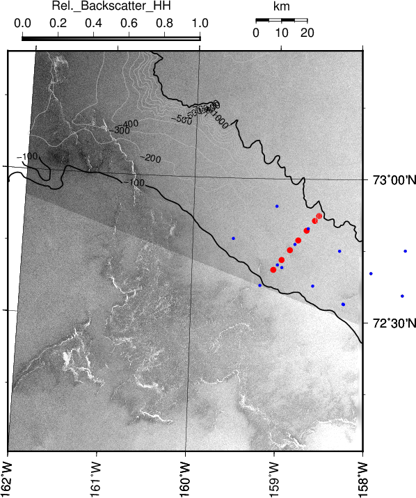
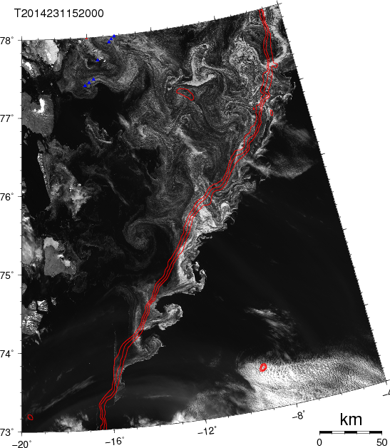
Map northern Chukchi Sea with mooring locations (red and blue symbols), contours of bottom topography, and radar backscatter from space. Slightly darker shades especially in the bottom segment are interpreted as sea ice. The offset in grey scale between top and bottom is caused by me using different numbers for two different data segments to bring the data into a range that varies between 0 and 1.
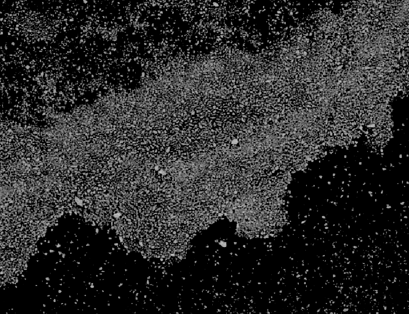
The image above is my first attempt to determine, if our planned mooring deployment locations are free of sea ice or not. The darker tones of gray are sea ice with the white spots probably thicker or piled-up ridges of rougher sea ice. The speckled gray surface to the north is probably caused by surface waves and other “noise” that are pretty random. There is a data point ever 40 meters in this image. It also helps to compare these very high-resolution ice data with products that the US National Ice Center (NIC) and the National Weather Service provide:
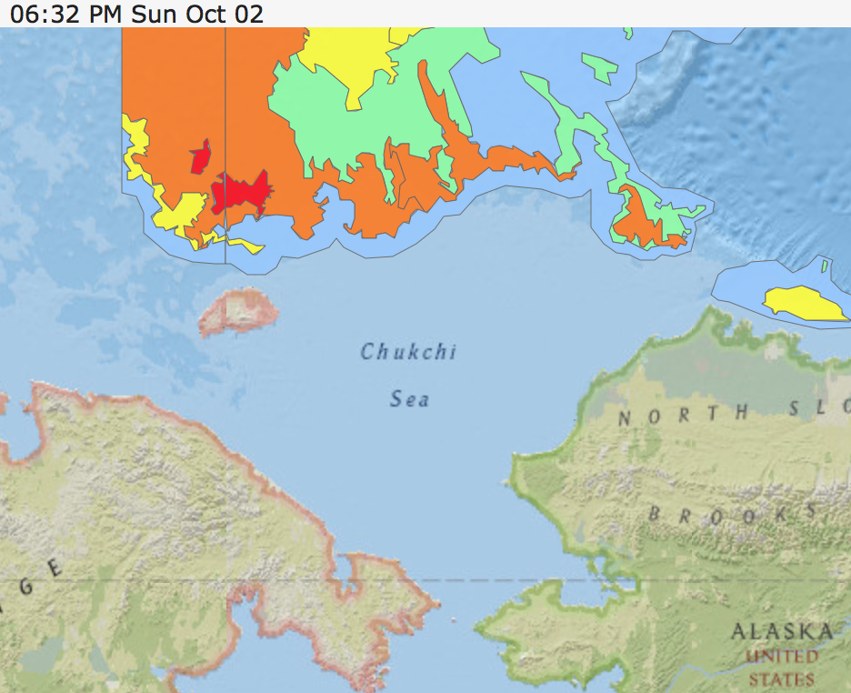
Ice Chart of the Alaska office of the National Weather Service
The above is a wonderful map for general orientation, but it is not good or detailed enough to navigate a ship through the ice. The two maps agree, however, my patch of ice to the south of the moorings are represented as the orange/green patch on the top right (north-east). The orange means that 70-80% of the area is covered by ice and this ice is thicker than 1.2 meters and thus too thick for our ship to break through, but there are always pathways through ice and those can be found with the 40-m resolution maps.
In summary, on Sept.-29, 2016 all our moorings are in open water, but this can change, if the wind moves this math northward. So we are also watching the winds and here I like the analyses of Government Canada
Surface weather analysis from Government Canada for Oct.-2, 2016. The map of surface pressure is centered on the north pole with Alaska at the bottom, Europe on the top, Greenland on the right, and Siberia on the left.
It shows a very low pressure center over Siberia to the south-west and a high pressure center over Arctic Canada to our north-east. This implies a strong wind to the north in our study area. So the ice edge will move north into our study area. If the High moves westward, we would be golden, but the general circulation at these latitudes are from west to east, that is, the Low over Siberia will win and move eastward strengthening the northward flow. That’s the bad news for us, but we still have almost 2 weeks before we should be in the area to start placing our fancy ocean moorings carefully into the water below the ice.
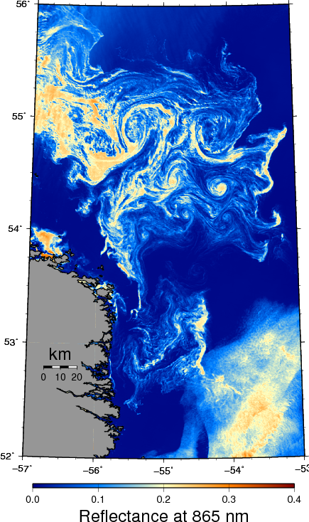
While this “operational” stuff motivated me to dive into the satellite radar data that can “see” through clouds and fog, I am most excited about the discovery that the radar data from the European Space Agency are easy to use with a little clever ingenuity and a powerful laptop (2.5 MHz Mac PowerBook). For example, this hidden gems appeared in the Chukchi Sea a few days earlier:
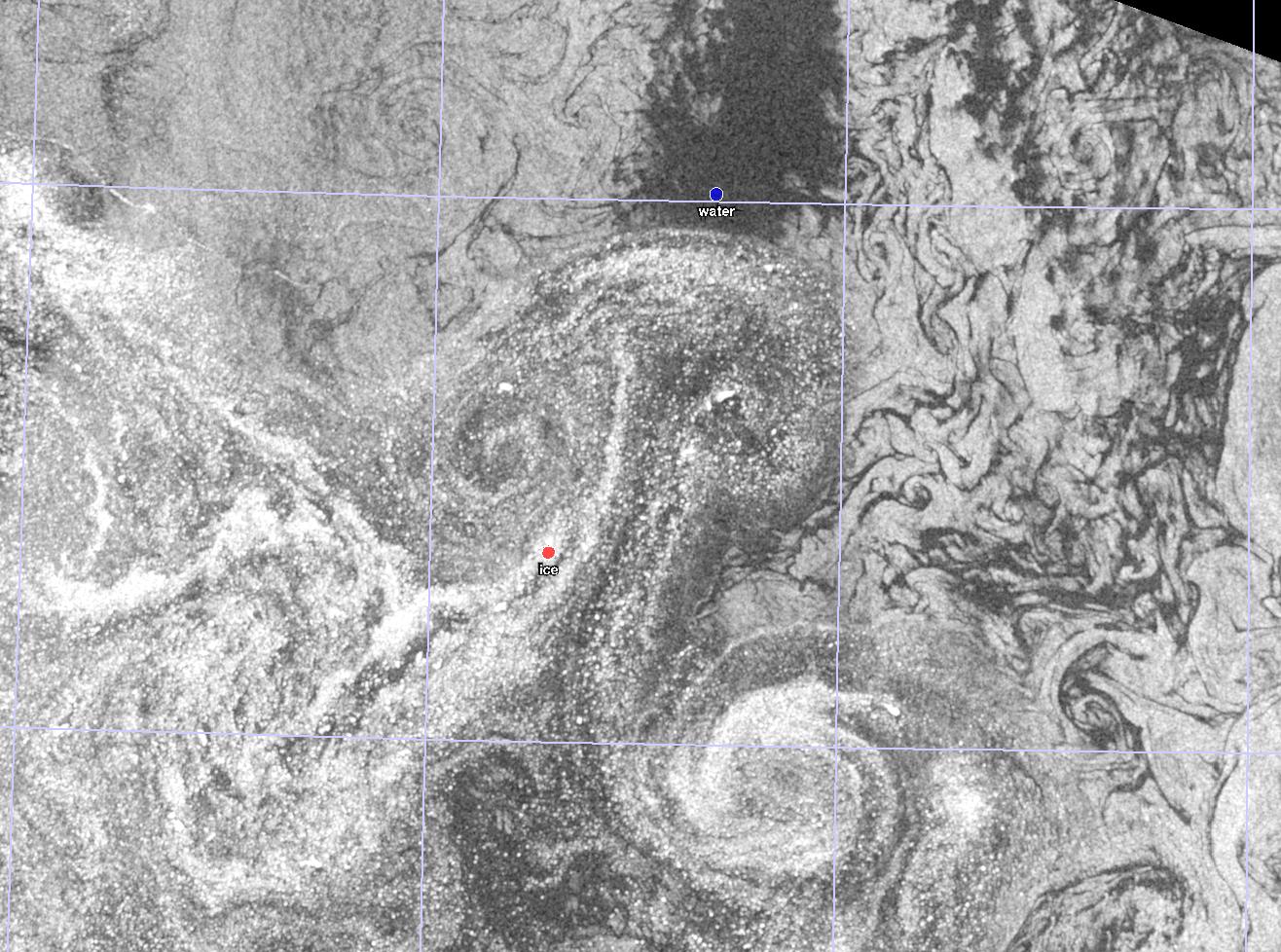
Close-up of the ice edge in the northern Chukchi Sea on Sept.-23, 2016. The mushroom cloud traced by sea ice and associated eddies are about 10-20 km across.
It is a piece of art, nature’s way to paint the surface of the earth only to destroy this painting the next minute or hour or day to make it all anew. It reminds me of the sand-paintings of some Native American tribes in the South-West of the USA that are washed away the moment they are finished. Here the art is in the painting, just as the pudding is in the eating, and the science is the thinking.

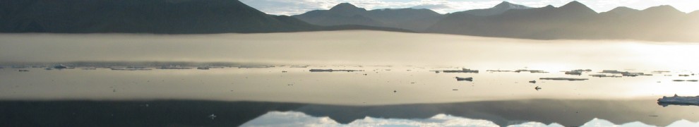
![Ice fields seen in Labrador Current April 6, 2008 from a plane. [Photo Credit: Daniel Schwen]](https://icyseas.org/wp-content/uploads/2013/05/labrador_current.jpg)


