I spent 6 weeks aboard the German research icebreaker R/V Polarstern last year leaving Tromso in Norway in early September and returned to Bremerhaven, Germany in October. We successfully recovered ocean sensors that we had deployed more than 3 years before. It felt good to see old friends, mates, and sensors back on the wooden deck. Many stories, some mysterious, some sad, some funny and happy could be told, but today I am working on some of the data as I reminisce.
-
- University of Delaware mooring returning to the surface Sept.-29, 2017 off North Greenland.
-

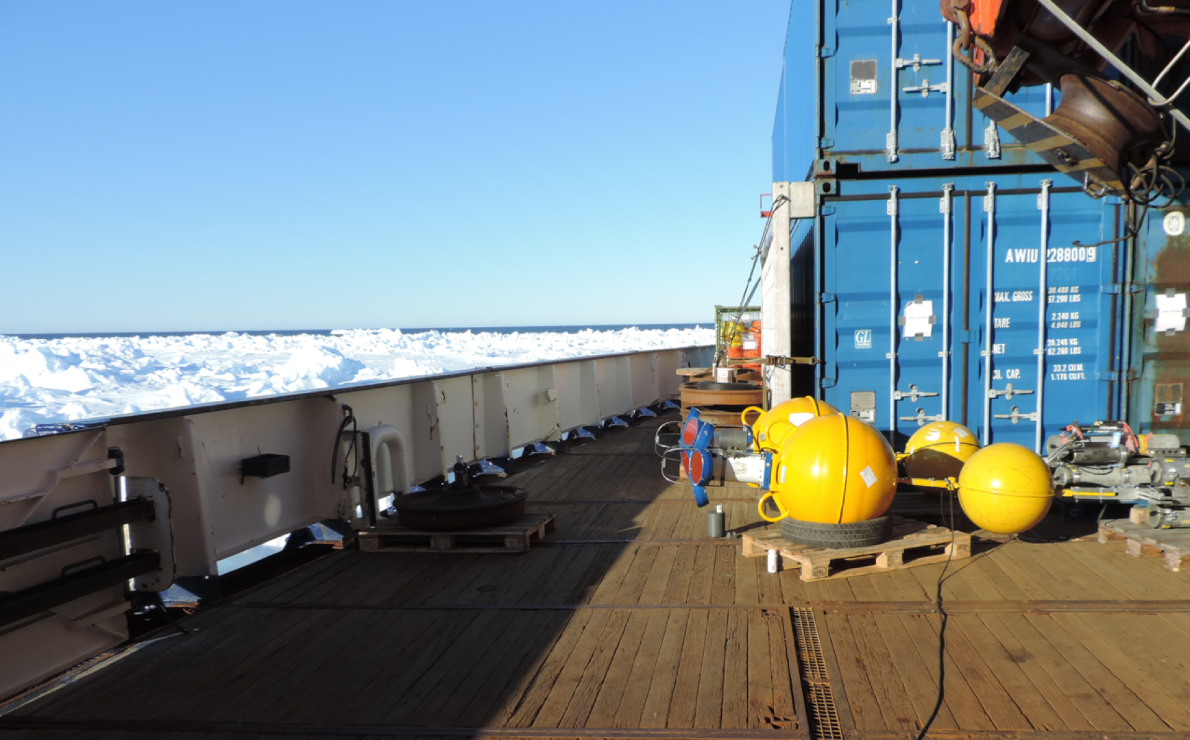
- University of Delaware mooring hoisted onto the deck of R/V Polarstern on Sept.-29, 2017.
-

- Mandy was here painting in 2014, but not in 2017.
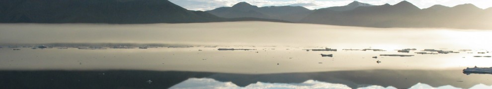
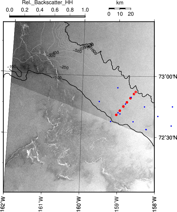
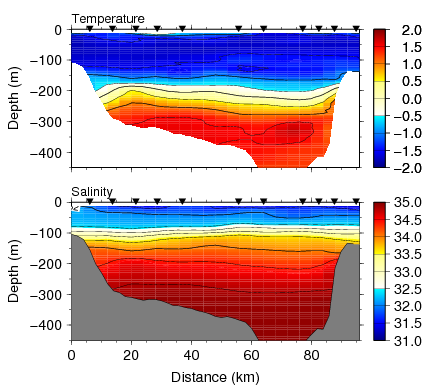
The location is North-East Greenland where Fram Strait connects the Arctic Ocean to the north with the Atlantic Ocean in the south. We worked mostly on the shallow continental shelf areas where water depths vary between 50 and 500 meters. The map shows these areas in light bluish tones where the line shows the 100 and 300 meter water depth. Fram Strait is much deeper, more than 2000 meters in places. I am interested how the warm Atlantic water from Fram Strait moves towards the cold glaciers that dot the coastline of Greenland in the west.
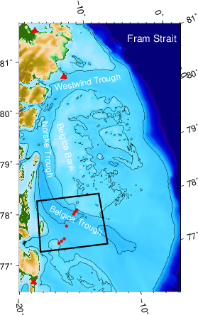
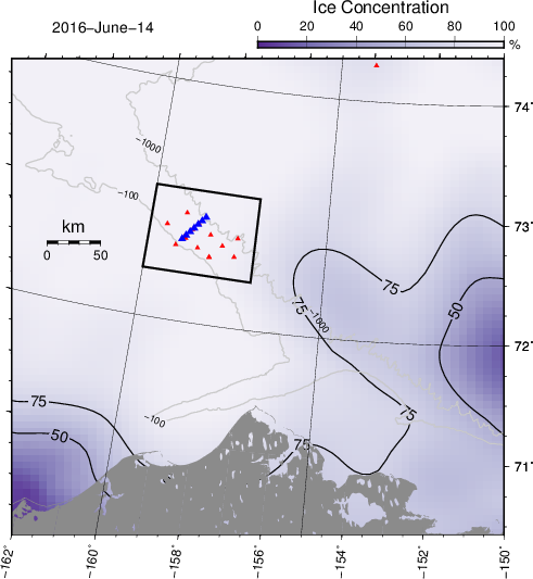
Map of study area with 2014-16 mooring array in box near 78 N across Belgica Trough. Red triangles place weather data from Station Nord (81.2 N), Henrik Kr\o yer Holme (80.5 N), and Danmarkhaven (76.9 N). Black box indicates area of mooring locations.
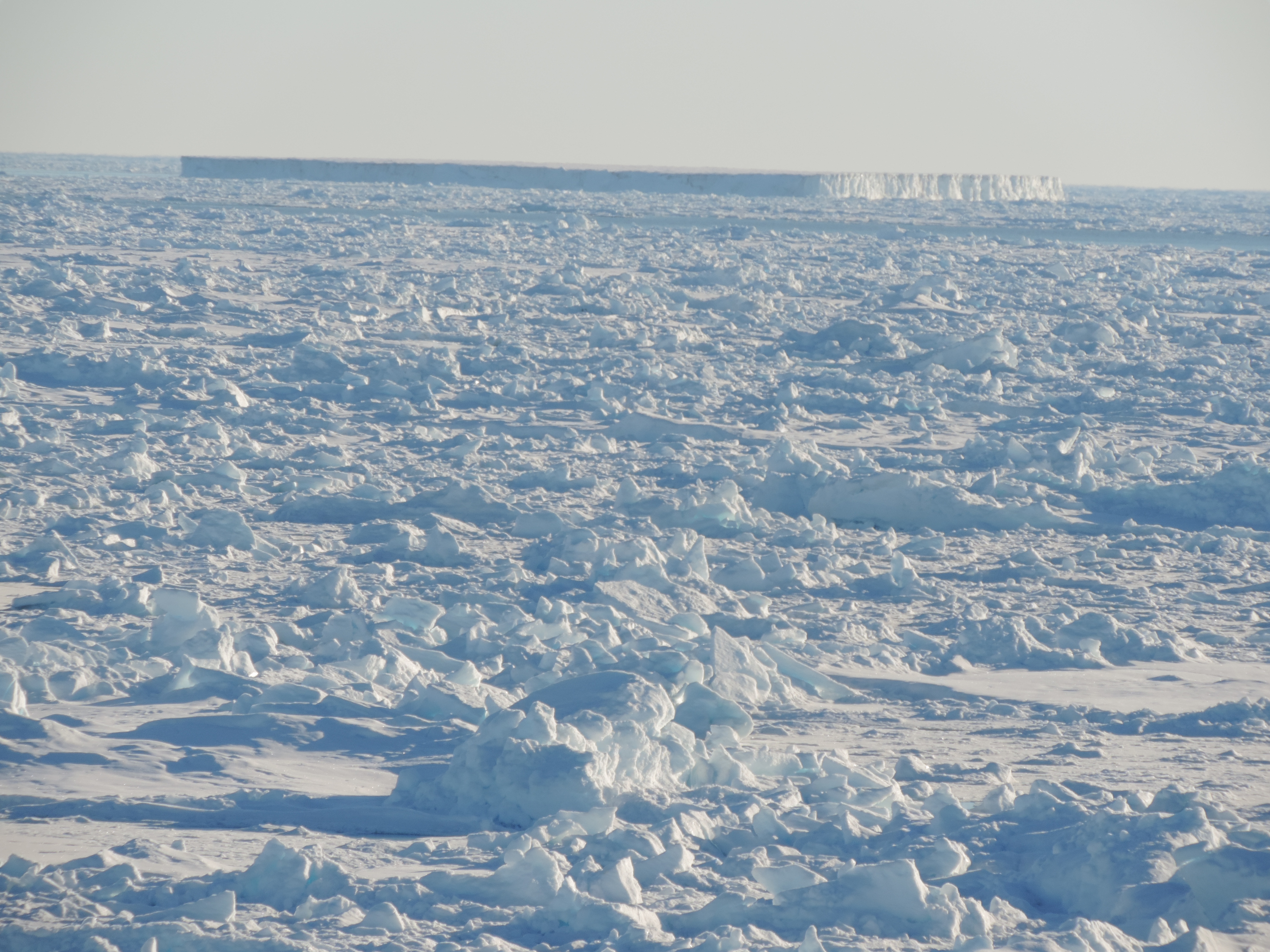
There is also ice, lots of sea icebergs, and ice islands that we had to navigate. None of it did any harm to our gear that we moored for 1-3 years on the ocean floor that can and often is scoured by 100 to 400 meter thick ice from glaciers, however, 2-3 meter thick sea ice prevented us to reach three mooring locations this year and our sensors are still, we hope, on the ocean floor collecting data.
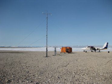
Ahhh, data, here we come. Lets start with the weather at this very lonely place called Henrik Krøyer Holme. The Danish Meteorological Institute (DMI) maintains an automated weather station that, it seems, Dr. Ruth Mottram visited and blogged about in 2014 just before we deployed our moorings from Polarstern back in 2014:
Weather station on Henrik Kroeyer Holme [Credit: Dr. Ruth Mottram, DMI]
It was a little tricky to find the hourly data and it took me more than a day to process and graph it to suit my own purposes, but here it is

Winds (A) and air temperature (B) from an automated weather station at Henrik Kroeyer Holme from 1 June, 2014 through 31 August, 2016. Missing values are indicated as red symbols in (A).
The air temperatures on this island are much warmer than on land to the west, but it still drops to -30 C during a long winter, but the end of July it reaches +5 C. The winds in summer (JJA for June, July, and August) are weak and variable, but they are often ferociously strong in winter (DJF for December, January, February) when they reach almost 30 meters per second (60 knots). The strong winter winds are always from the north moving cold Arctic air to the south. The length of each stick along the time line relates the strength of the winds, that is, long stick indicates much wind. The orientation of each stick indicates the direction that the wind blows, that is, a stick vertical down is a wind from north to south. I use the same type of stick plot for ocean currents. How do these look for the same period?
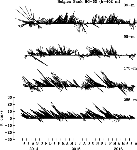
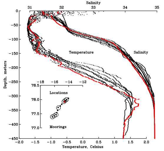
Ocean current vectors at four selected depths near the eastern wall of Belgica Trough. Note the bottom-intensified flow from south to north. A Lanczos low-pass filter removes variability at time scales smaller than 5 days to emphasize mean and low-frequency variability.
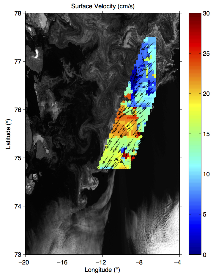
Ocean currents and winds have nothing in common. While the winds are from north to south, the ocean currents are usually in the opposite direction. This becomes particular clear as we compare surface currents at 39 meters below the sea surface with bottom currents 175 or even 255 meters below the surface. They are much stronger and steadier at depth than at the surface. How can this be?

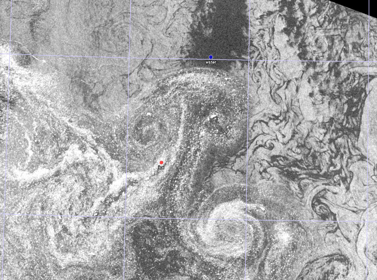
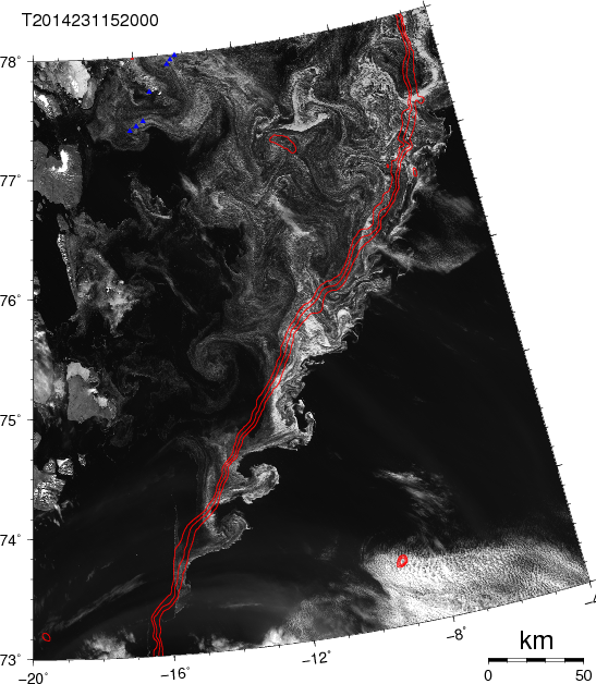
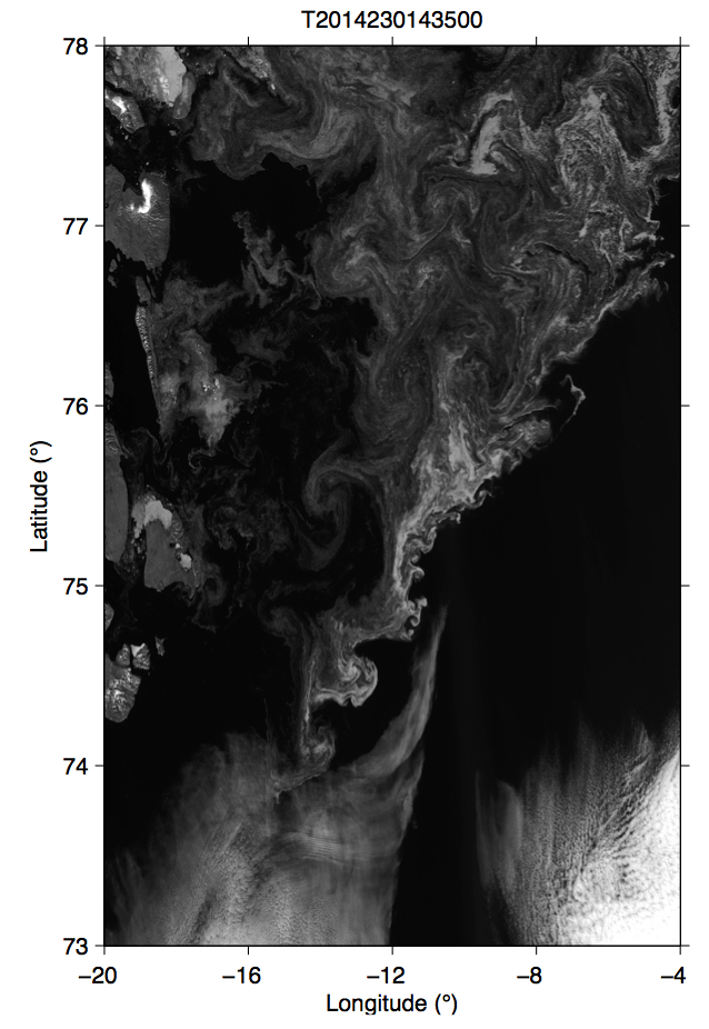
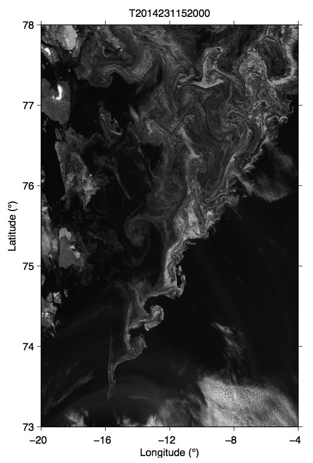
Image of study area on 15 June 2014 with locations (blue symbols) where we deployed moorings a few days before this satellite image was taken by MODIS Terra. The 100-m isobath is shown in red.
Well, recall that there is ice and for much of the year this sea ice is not moving, but is stuck to land and islands. This immobile winter ice protects the ocean below from a direct influence of the local winds. Yet, what is driving such strong flows under the ice? We need to know, because it is these strong currents at 200 to 300 meter depth that move the heat of warm and salty Atlantic waters towards coastal glaciers where they add to the melting of Greenland. This is what I am thinking about now as I am trying to write-up for my German friends and colleagues what we did together the last 3 years.
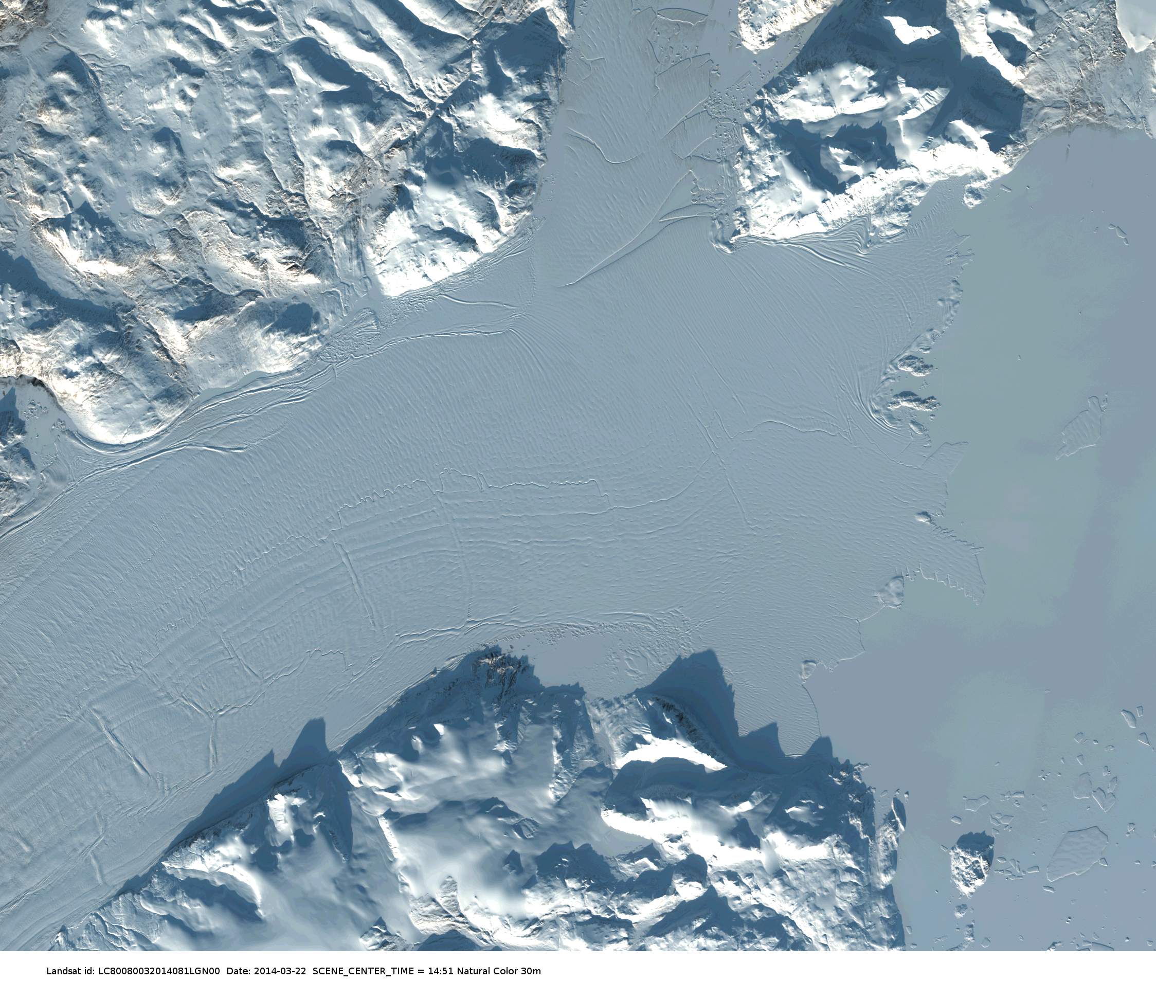
Oh yes, and we did reach the massive terminus of 79 North Glacier (Nioghalvfjerdsfjorden) that features the largest remaining floating ice shelf in Greenland:
We recovered ocean moorings from this location also, but this is yet another story that is probably best told by scientists at the Alfred-Wegener-Institute who spent much time and treasures to put ship, people, and science on one ship. I am grateful for their support and companionship at sea and hopefully all of next year in Bremerhaven, Germany.
![Icebreaker taking on waves on the stern during a fall storm in the Beaufort Sea in October 2004. [Photo Credit: Chris Linder, Woods Hole Oceanographic Institution]](https://icyseas.org/wp-content/uploads/2016/06/picture1.png)

