Icebreaker Polarstern reached its home port of Bremerhaven in Germany just before Orkan “Joshua” hit northern Germany hard. The ship returned after 3 month at sea with 48 crew and 46 scientists working on ocean biology, chemistry, and physics. The 7-week expedition from Svalbard to Greenland and back to Germany culminated 3 years of planing and preparations led by the Alfred Wegener Institute (AWI). As one of 46 scientists I stepped onto the ship almost two months ago in Longyearbyen. We planned to explore what moves ice and fresh Arctic water into the Atlantic Ocean with sensors to probe the coastal circulation. Analyzing these data, I will now live in Bremerhaven for a few months.
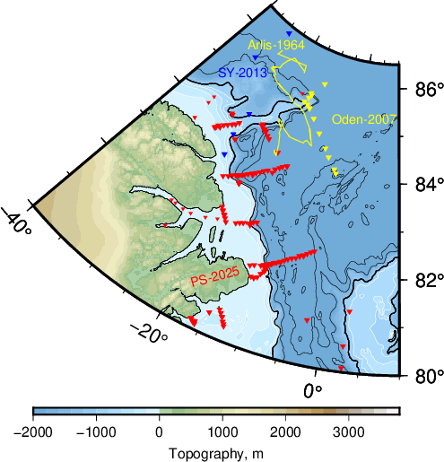
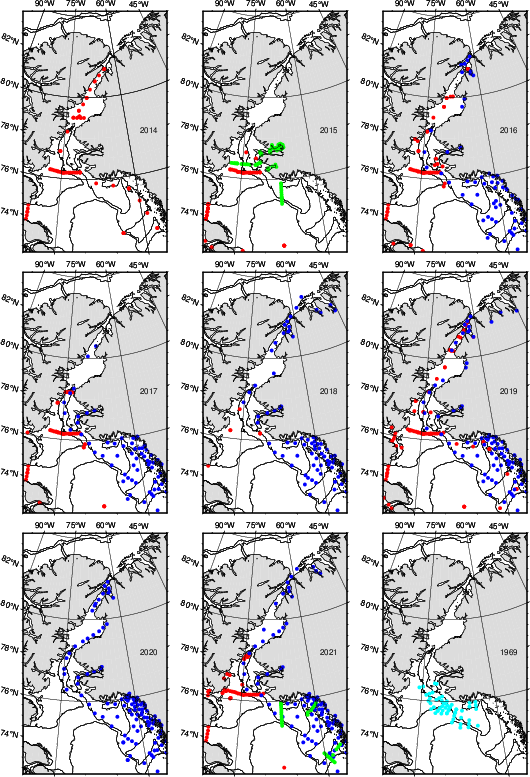
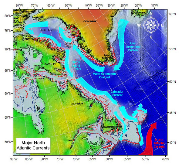
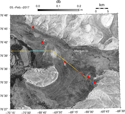
The map above shows where we went to the north of Greenland. I am coloring the coastal ocean shallower than 1000 m in light blue and the deeper ocean in dark blue. Our 2025 Polarstern data are the red symbols while yellow and blue symbols show data locations from 1964 ice island, 2007 icebreaker, and 2013 helicopter surveys. This area contains the last and thickest sea ice of the Arctic Ocean and prior ocean observations originate from floating ice islands that both the Soviet Union and the U.S.A. used during the Cold War 1947-91 such as the Arlis-1964 track (yellow line). Helicopter surveys collected a few data in 2013 (blue symbols) while the Swedish icebreaker Oden collected data along two lines farther offshore (yellow symbols).
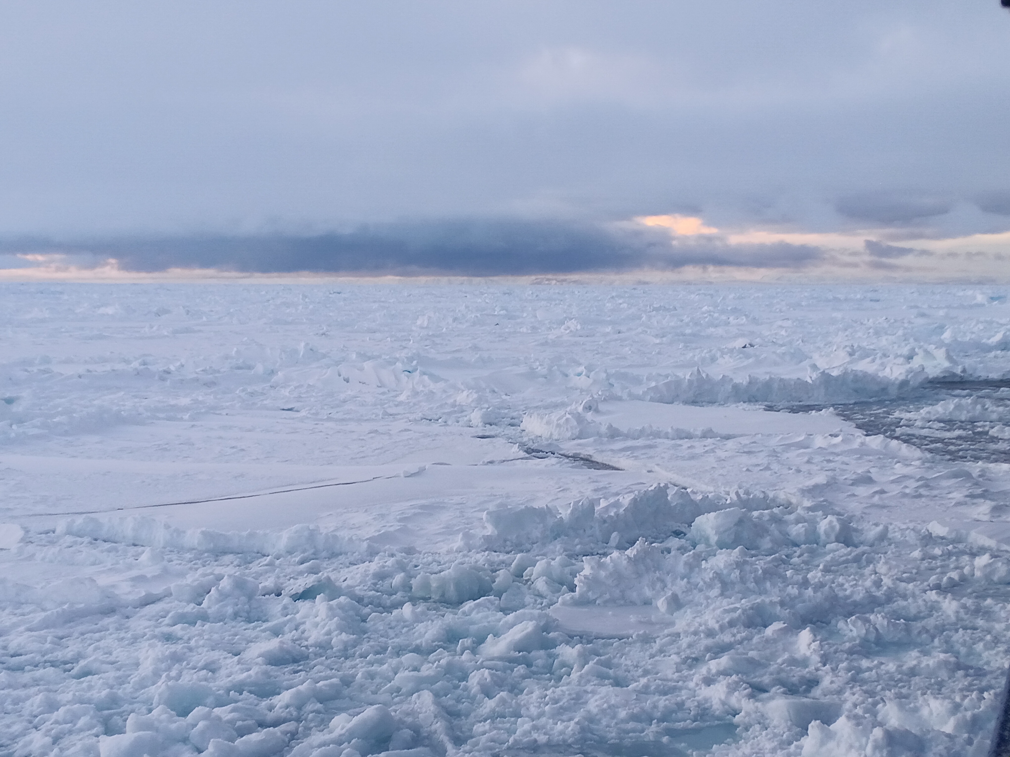
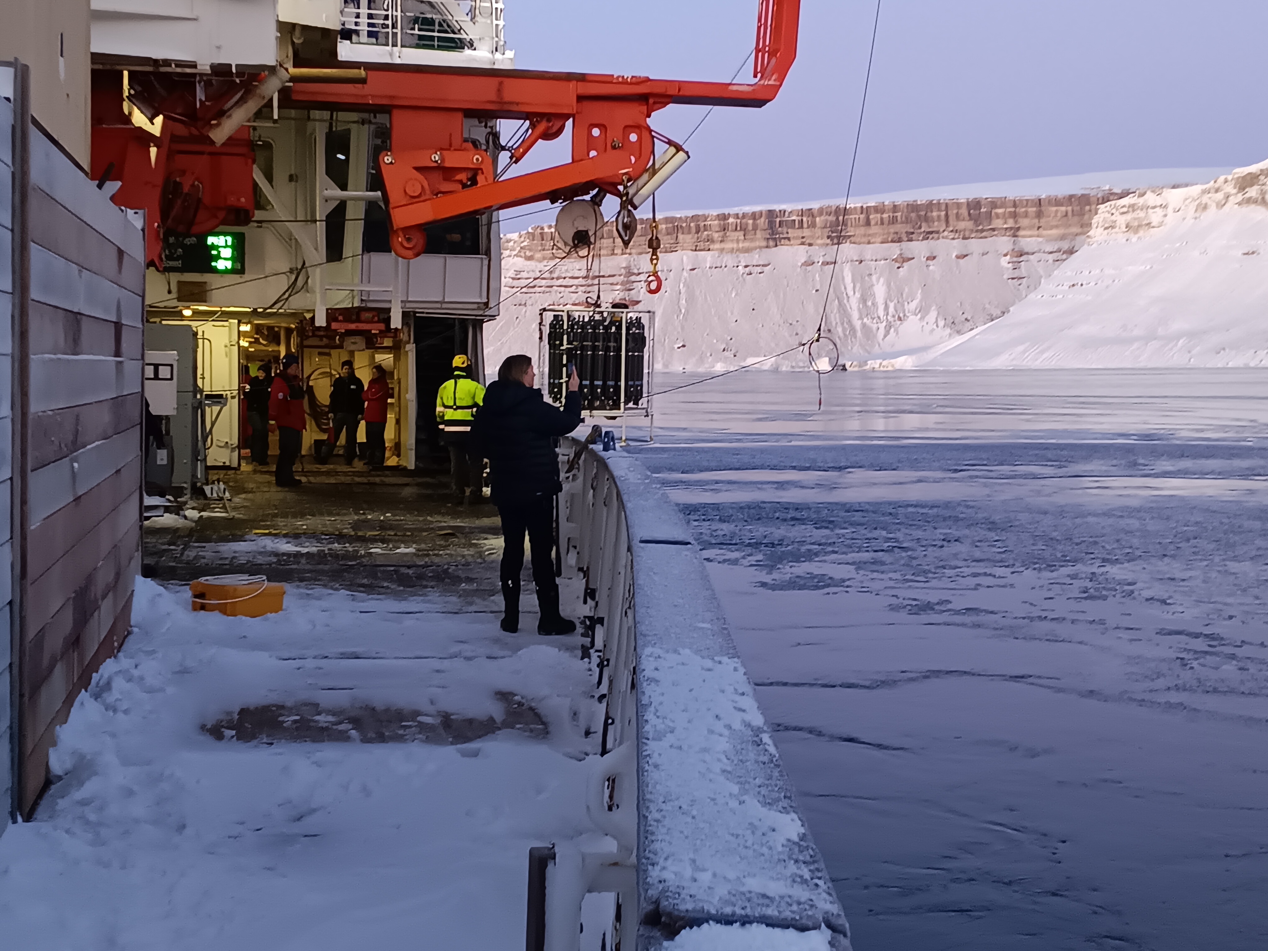
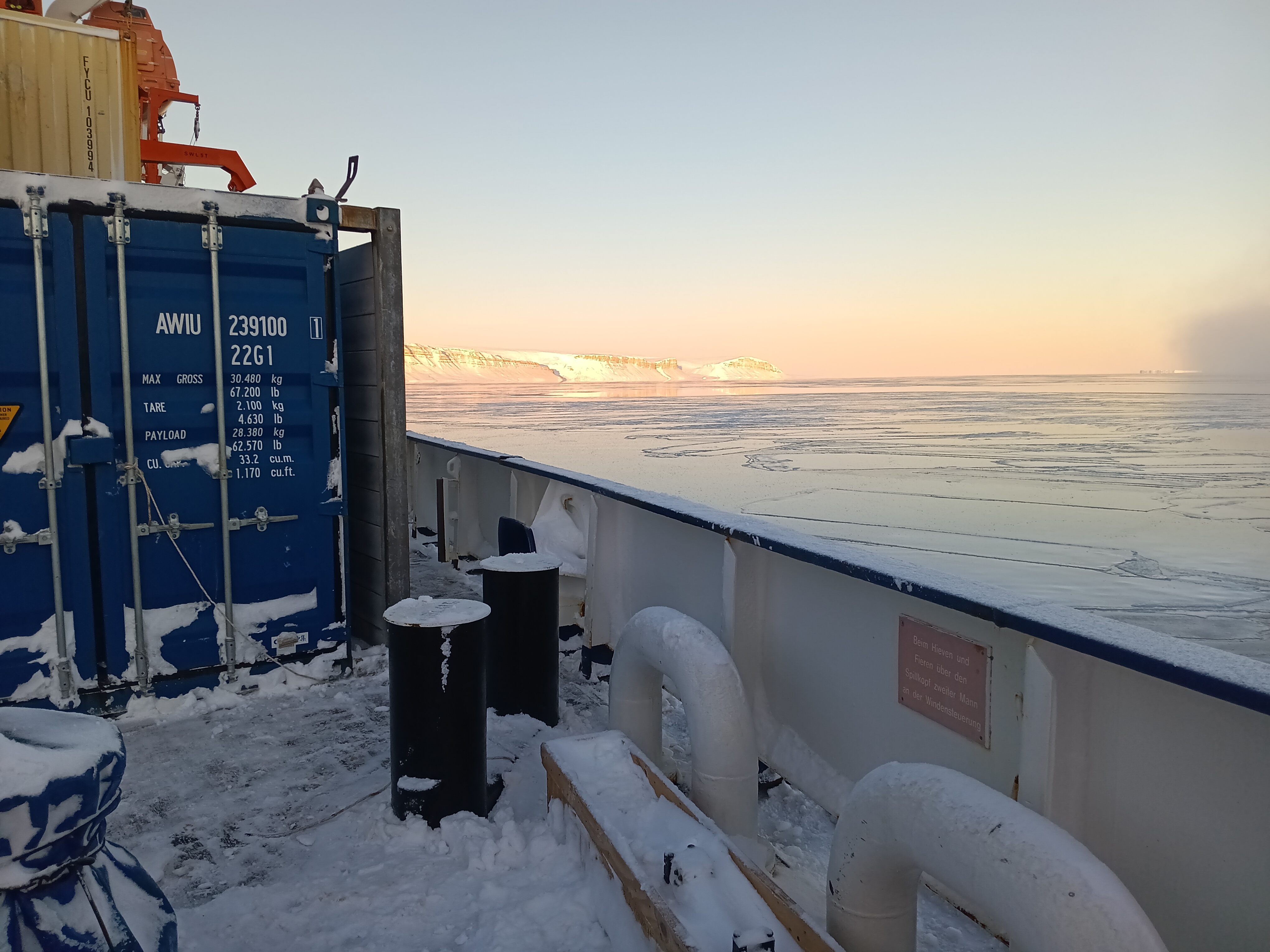
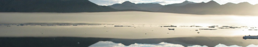
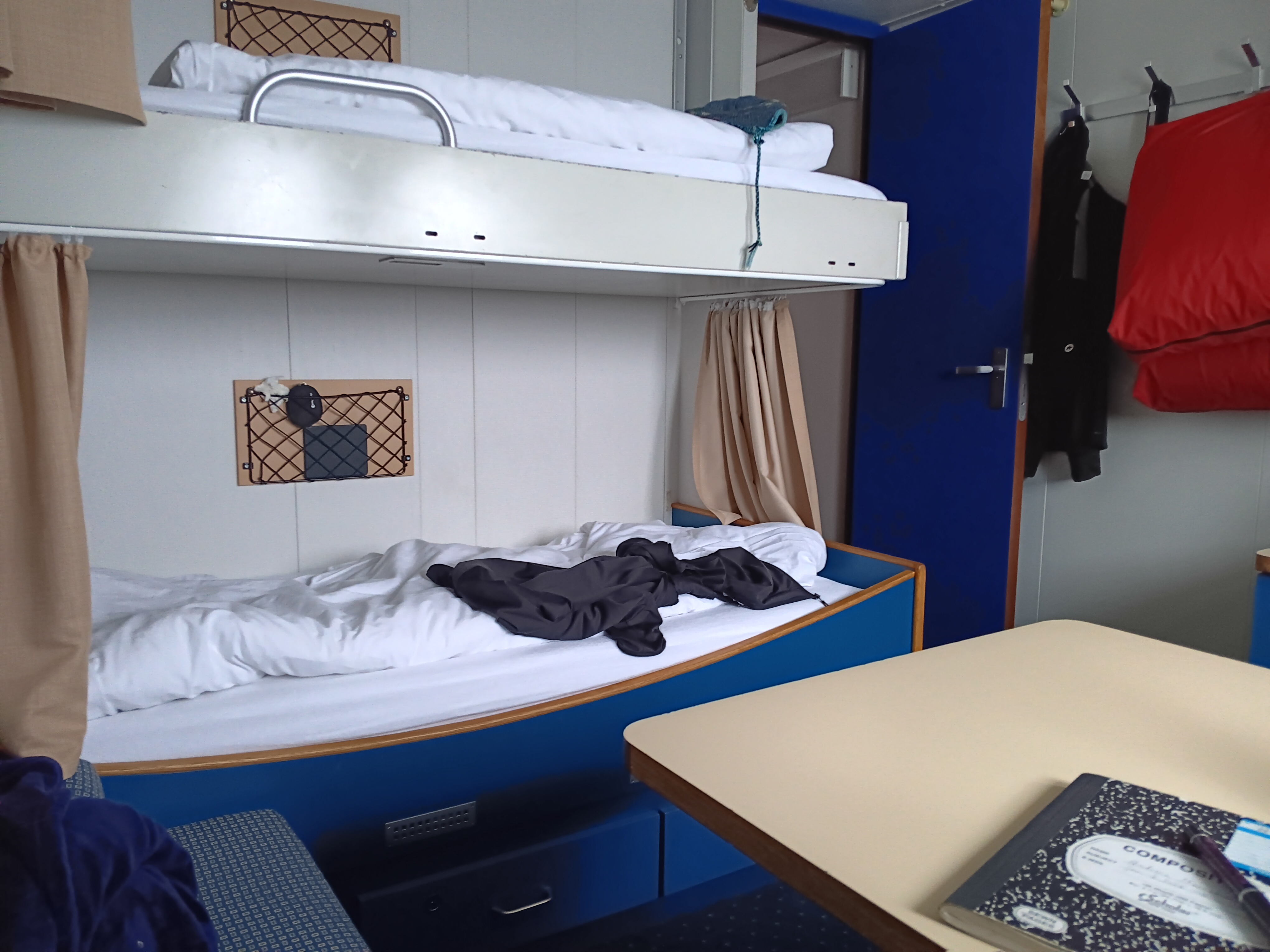
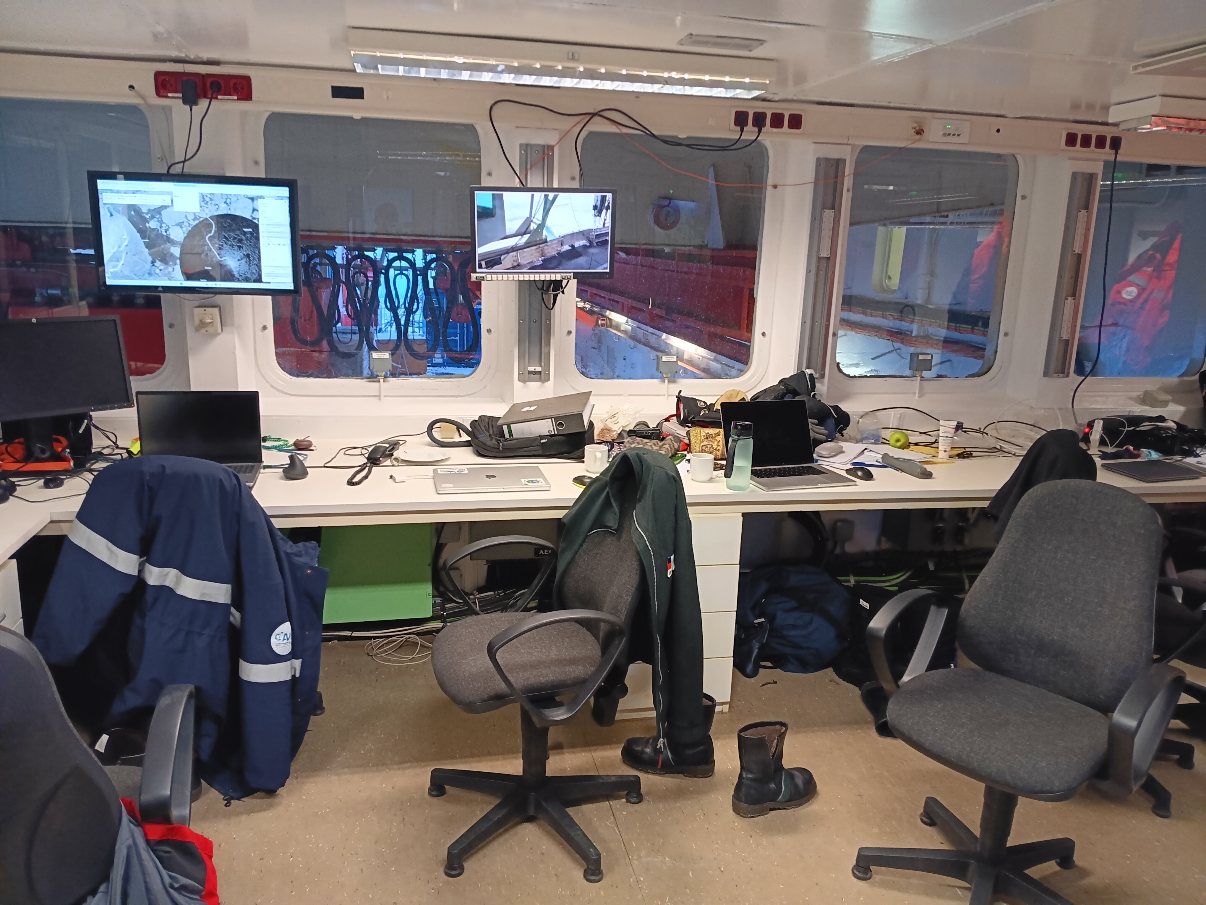
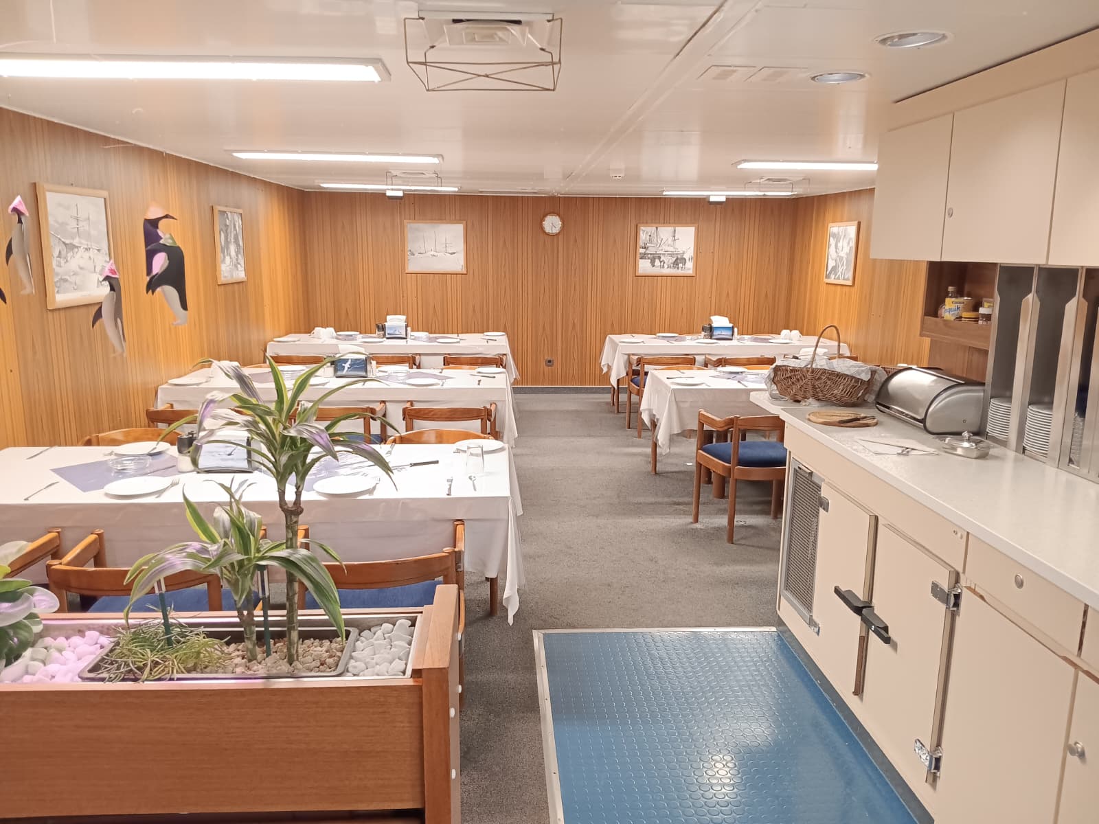
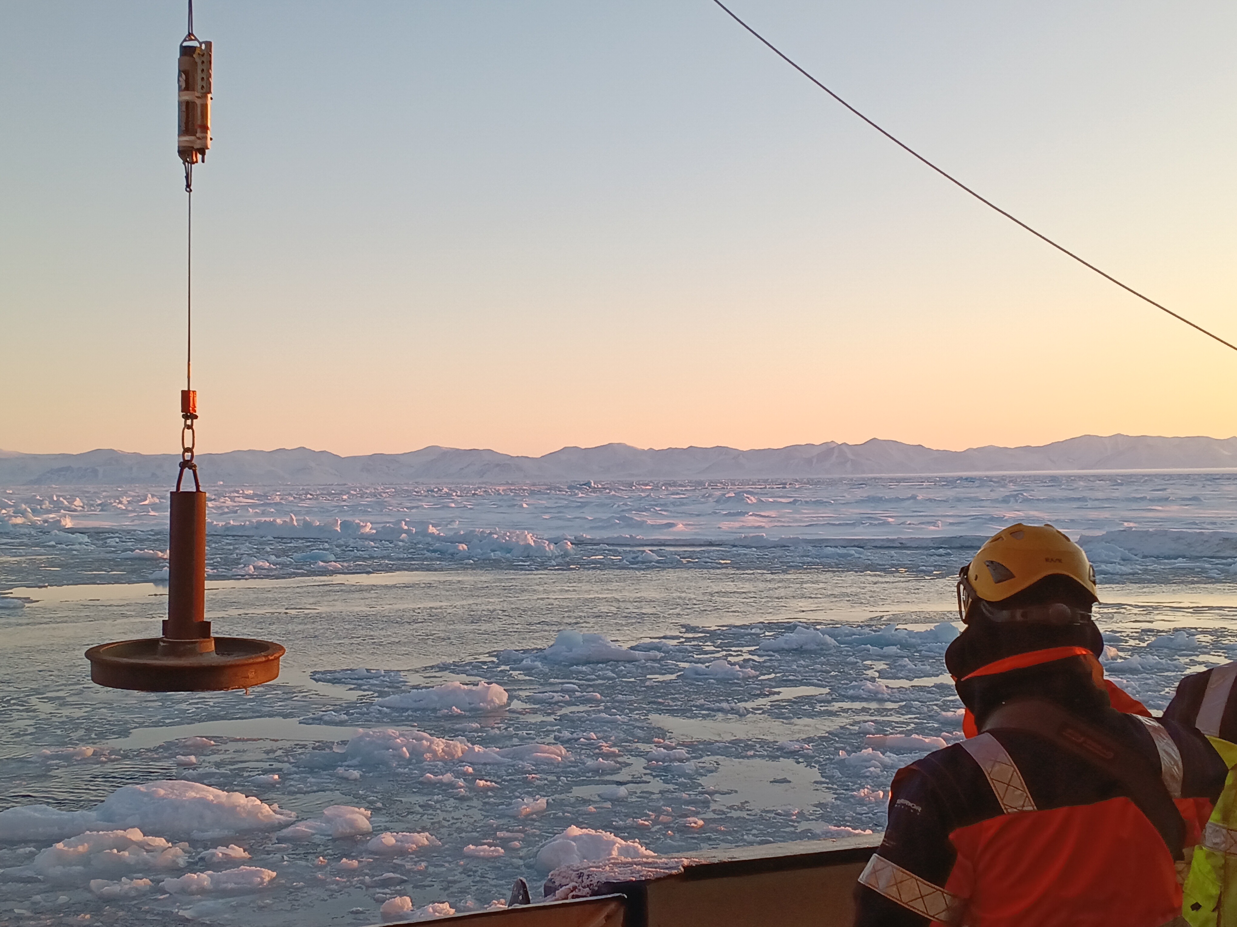
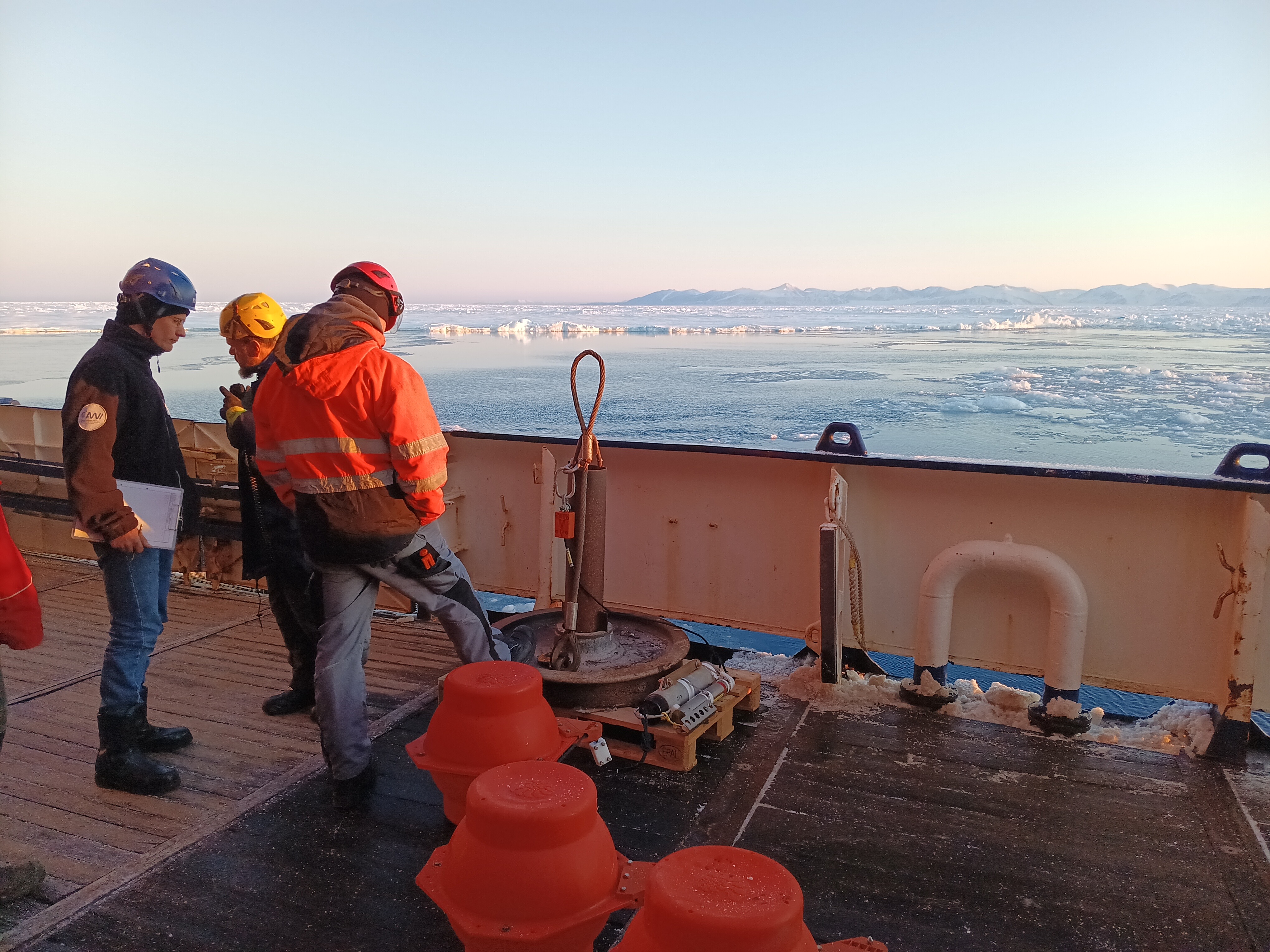
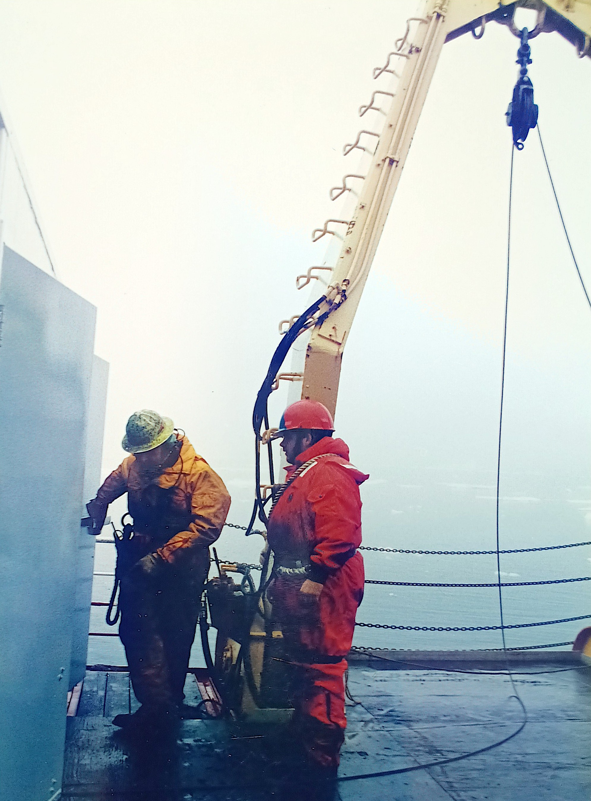
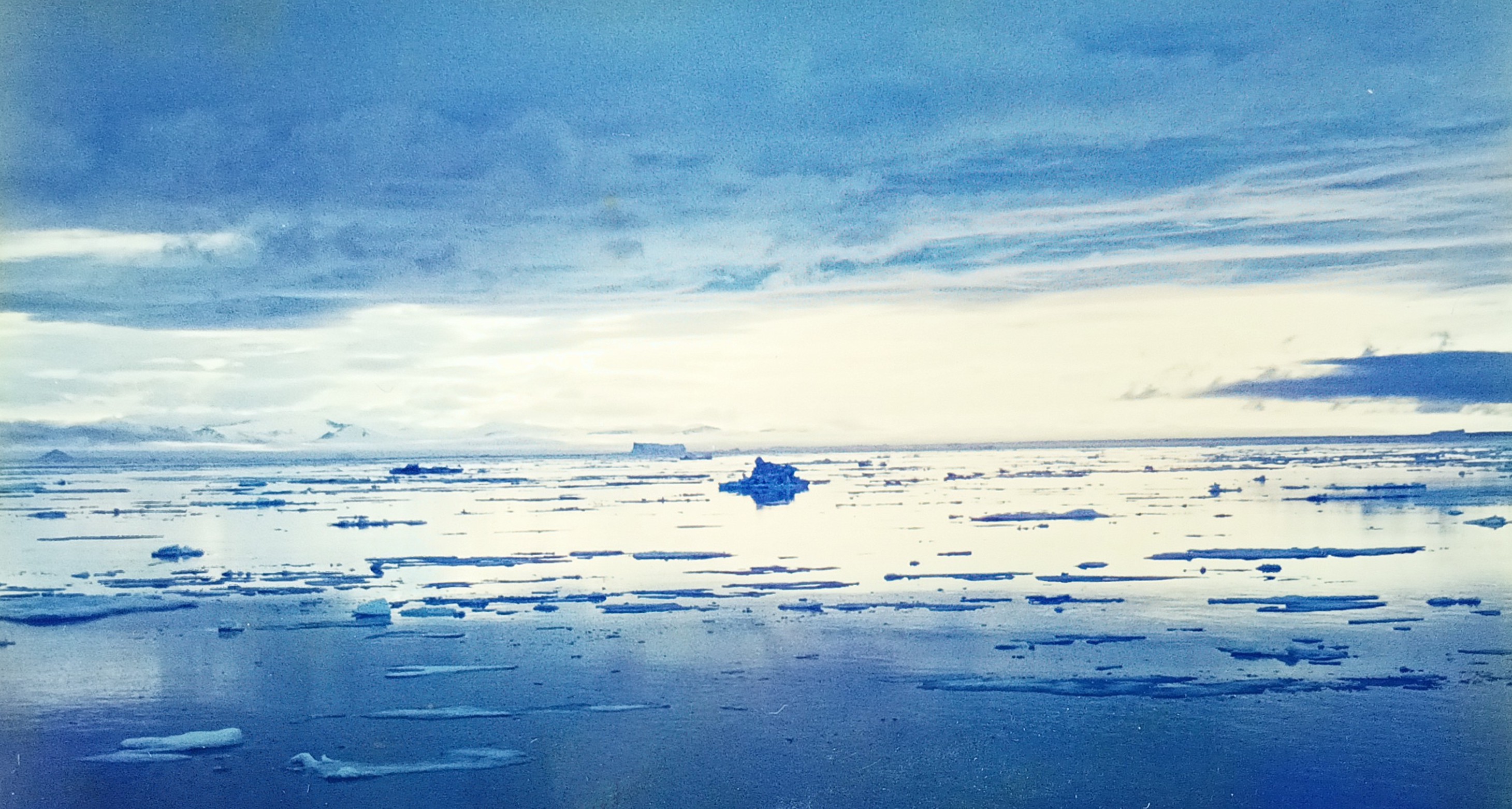
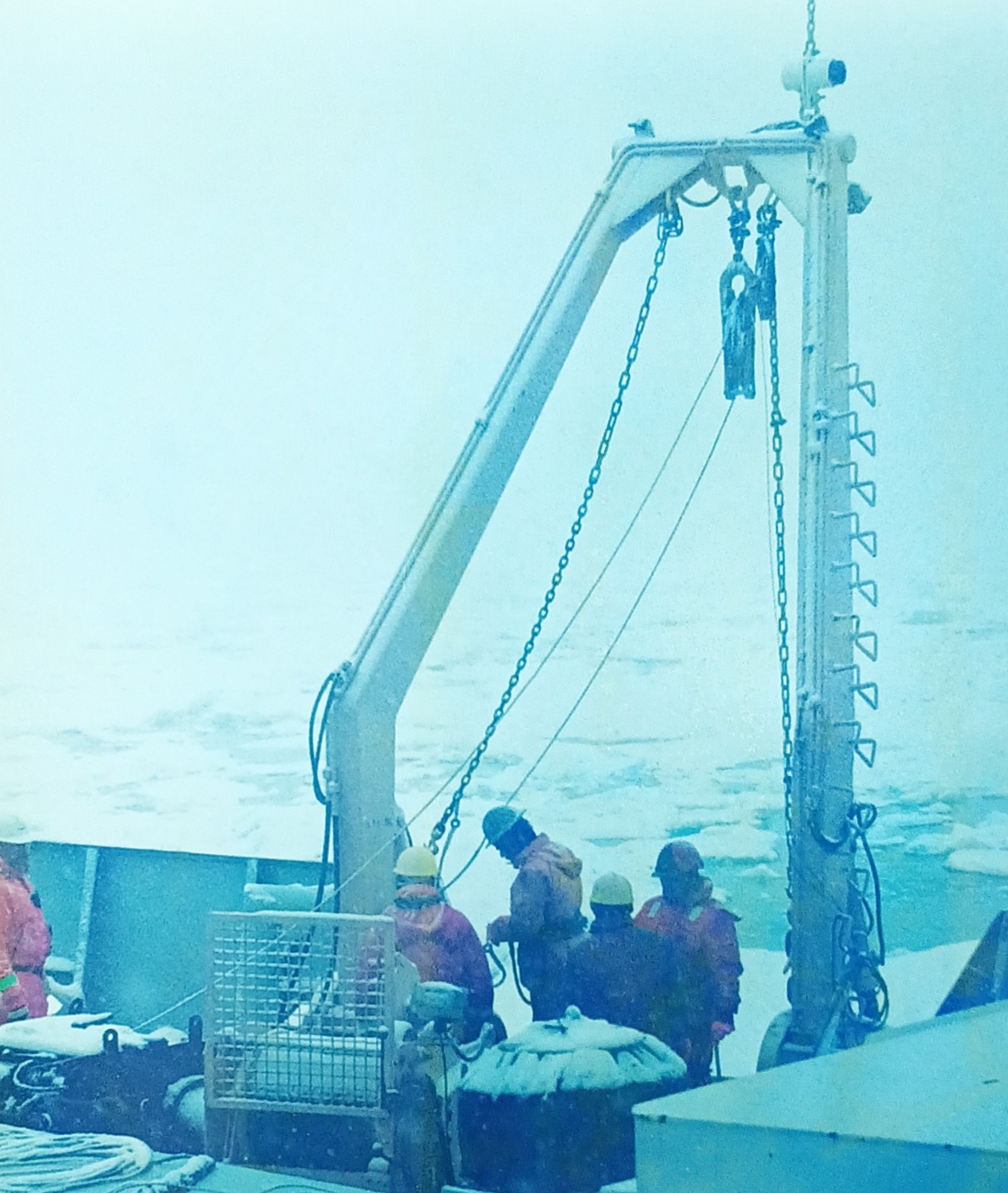
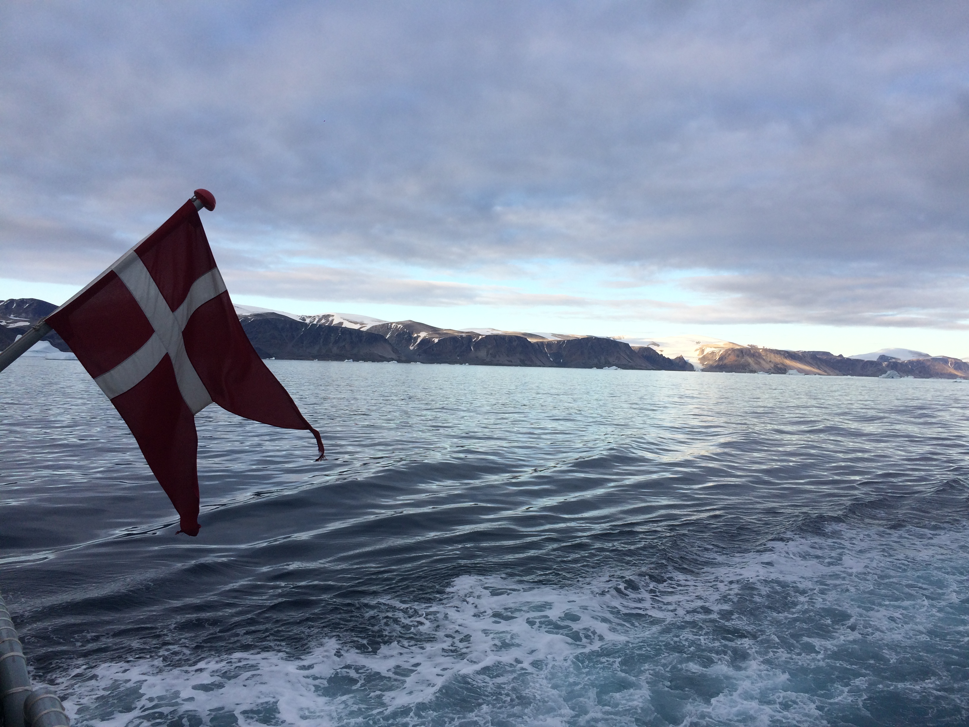
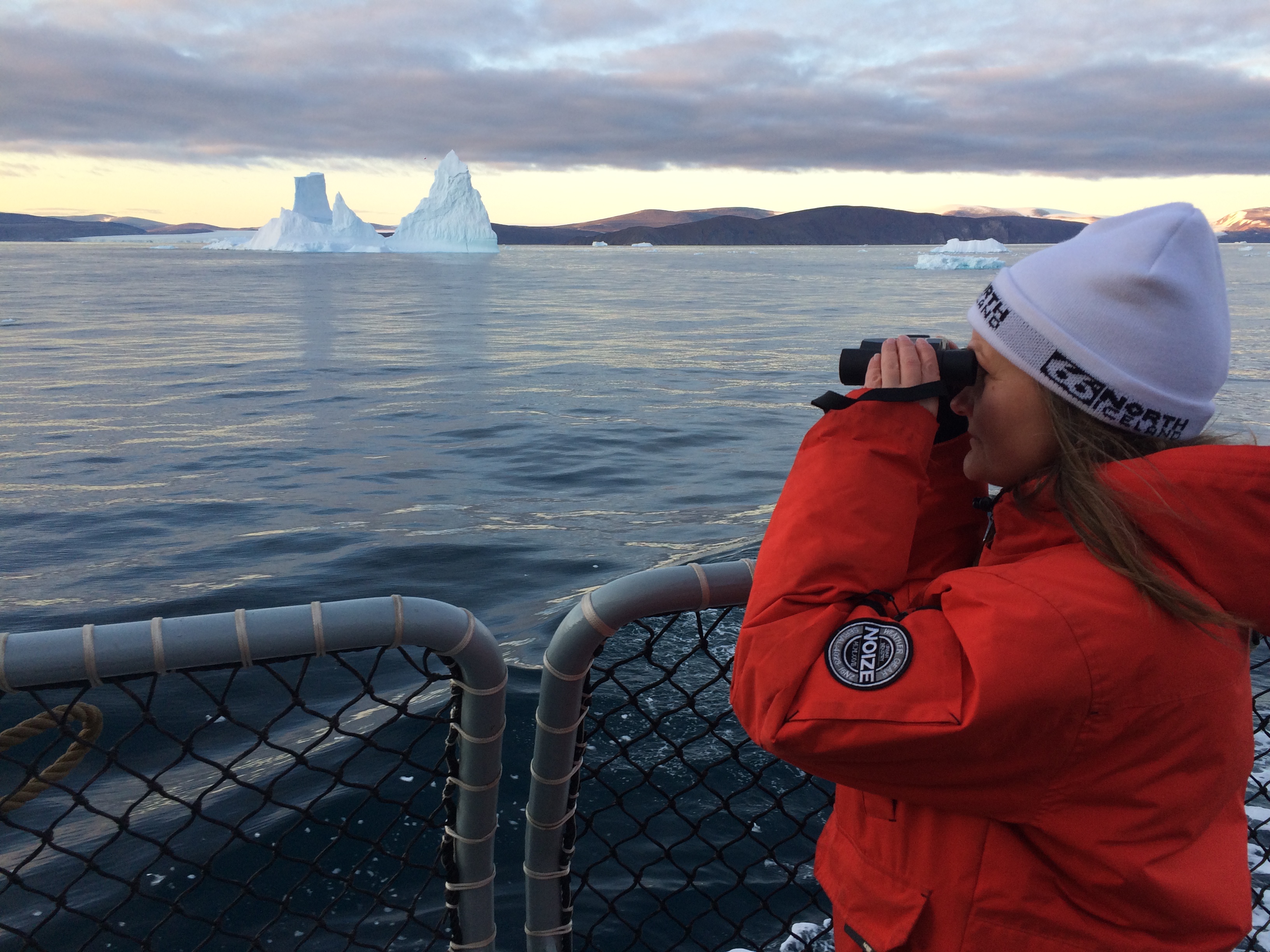
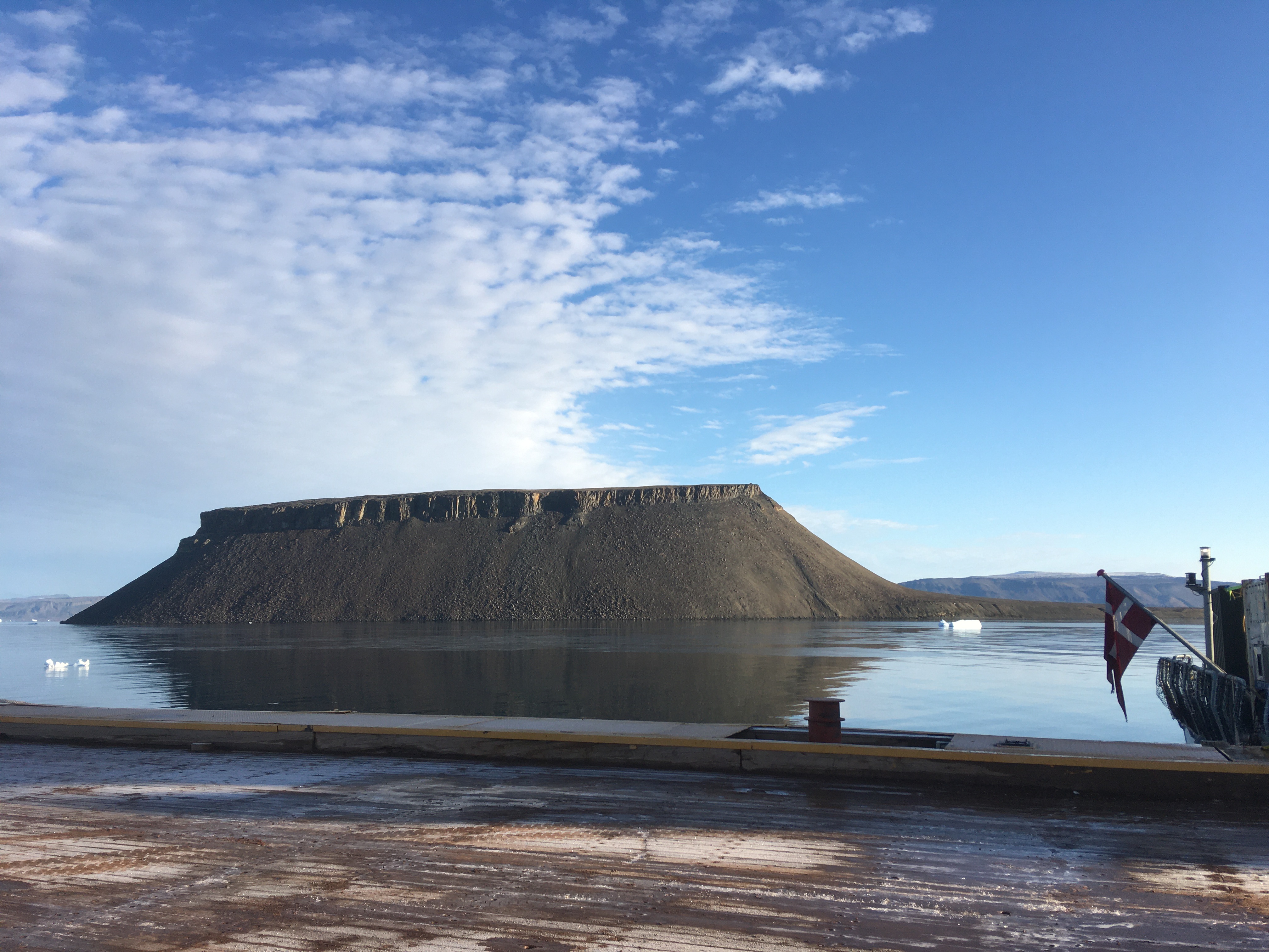
Now how does Greenland look from the ship? Well, there is always ice and it is always cold. The coldest days we had near the coast when the skies were clear. The coldest day we had -20 C, that is -4 F for my American friends, but most of the time we had clouds and storms with temperatures warmer at -12 C (10 F) with clouds and little visibility. It snowed alot and shoveling the ship’s deck was an almost daily chore. A relaxing “cruise” it was not. We worked sensors systems in the windy cold outside during all hours of the day and night. Pictures like the above were almost always taken during my 8 hours “off” that for me was from 08:00 to 16:00, because my shift was from 16:00 to 24:00. After a phone call to my wife after midnight and a peppermint tea to warm up, I slept from 01:00 to breakfast at 07:30. As almost all scientists aboard I shared my cabin with others, so there is not too much privacy. The photos below show my bunk bed (I slept atop), shared work spaces, and the rarely empty dining room. We often ate in shifts, too, because not all 50 people would fit the dining room in one sitting. So we often had 2 sittings. A comfortable living room was next door for desert, tea, coffee, games, and conversations.
Now what about science, you may ask. Here we made a major discovery, I felt. A mathematician used her craft to predict a coastal current to the north of Greenland that, I admit, made no sense to me as it contradicted 30+ years of training and intuition in which direction such currents would flow, that is, the coast should be on the right hand side looking in the direction of the flow. The curious thing was that to the north of Greenland it should go in the opposite direction, that is, with the coast on the left. In Claudia’s numerical computer model run for months on super computers, this current-in-the-wrong-direction was a both prominent and persistent feature. I always discarded it as an unrealistic feature of some computer code run amok. And yet, when we actually reach the coast of northern Greenland and I measure ocean currents from a ship sensor that runs 24/7 to tell me current speed and direction, here this weired or “wrong” current was. It screamed at me from the screen the moment I plotted the data and shared it with Claudia who was aboard with the comment: “Your model is right and my intuition was wrong. Your current is at the same location, the same speed, and in the same direction as your model said it would.” Furthermore, a distinct and separate way to estimate ocean currents from ocean temperature and salinity observations showed the exact same thing. That’s now two good complementary confirmation of the current that nobody has ever seen or measured … until now that we aboard Polarstern did so on Sept.-23, 2025:
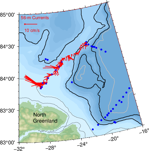
The map on the left shows our study area to the north of North Greenland. On it in red are sticks whose length indicate the speed or strength of the ocean current (at 56 meters below the surface) while its orientation gives the direction of the current. The light blue is shallow and dark blue is deep water as before. The current is sluggish offshore with a weak component to the south. In contrast, closest to the coast of North Greenland we find long sticks that point to towards the left (west by north-west). This is Claudia’s Coastal Current.
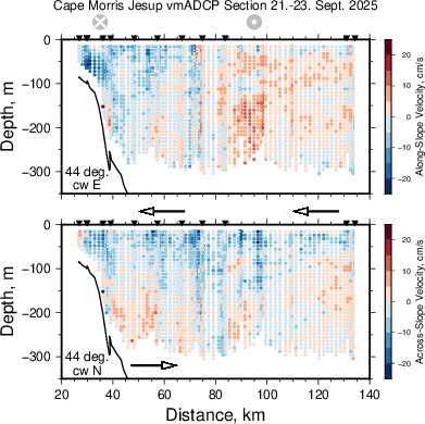
The two plots on the left provide more detail, as it shows how the current varies with depth and distance from the coast along a line from the coast towards offshore. The bottom of the shallow ocean is the black line from 100-m to 350-m meter at a distance of 20-40 km from the coast. The top-left panel shows the current (in colors) across the section where blue colors indicate currents flow into the page while red colors indicate currents that flow out of the page towards us viewing it with the coast on the left. The bottom-left panel shows the velocity component along the section with a flow that is mostly onshore near the surface.
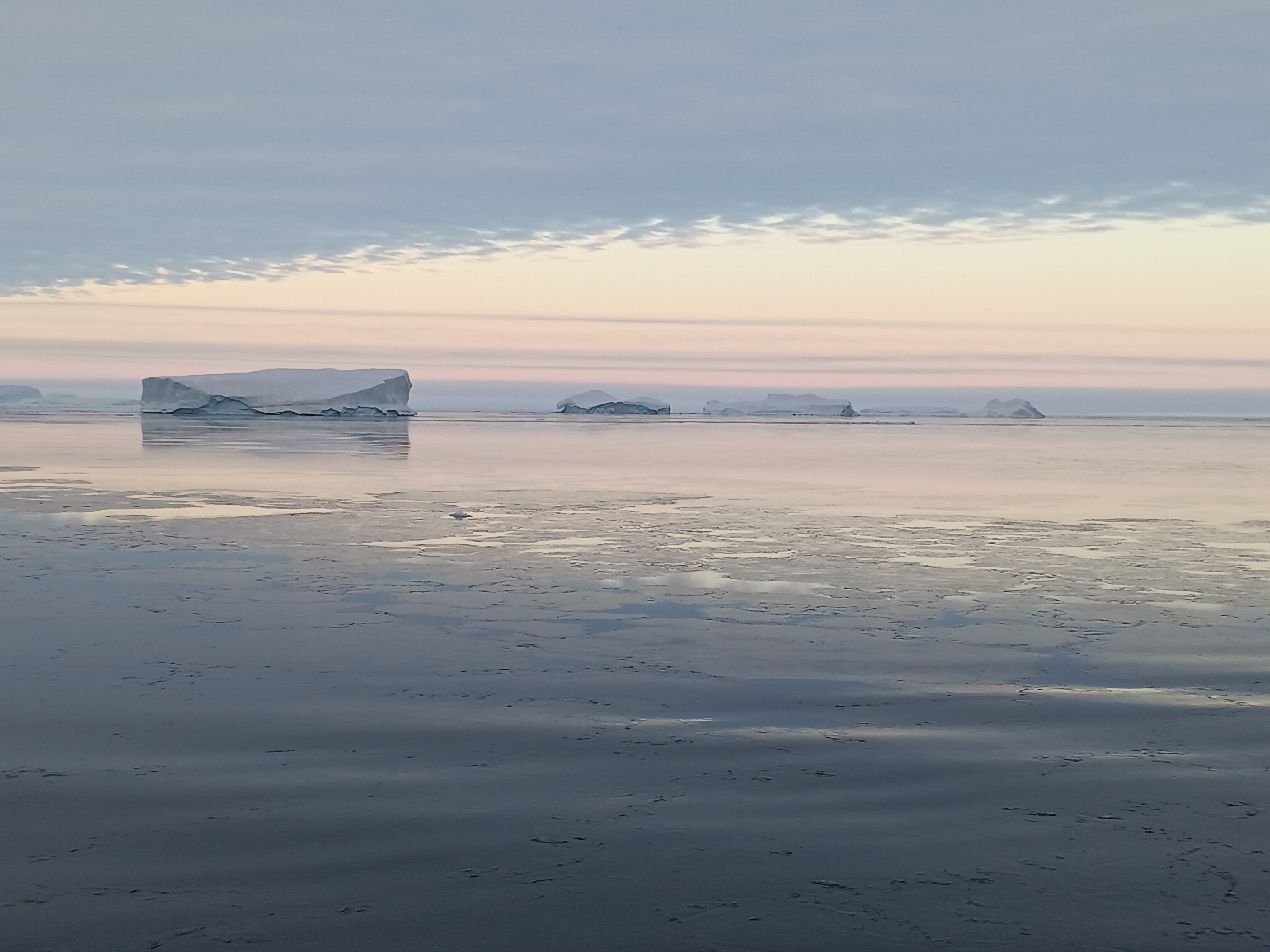
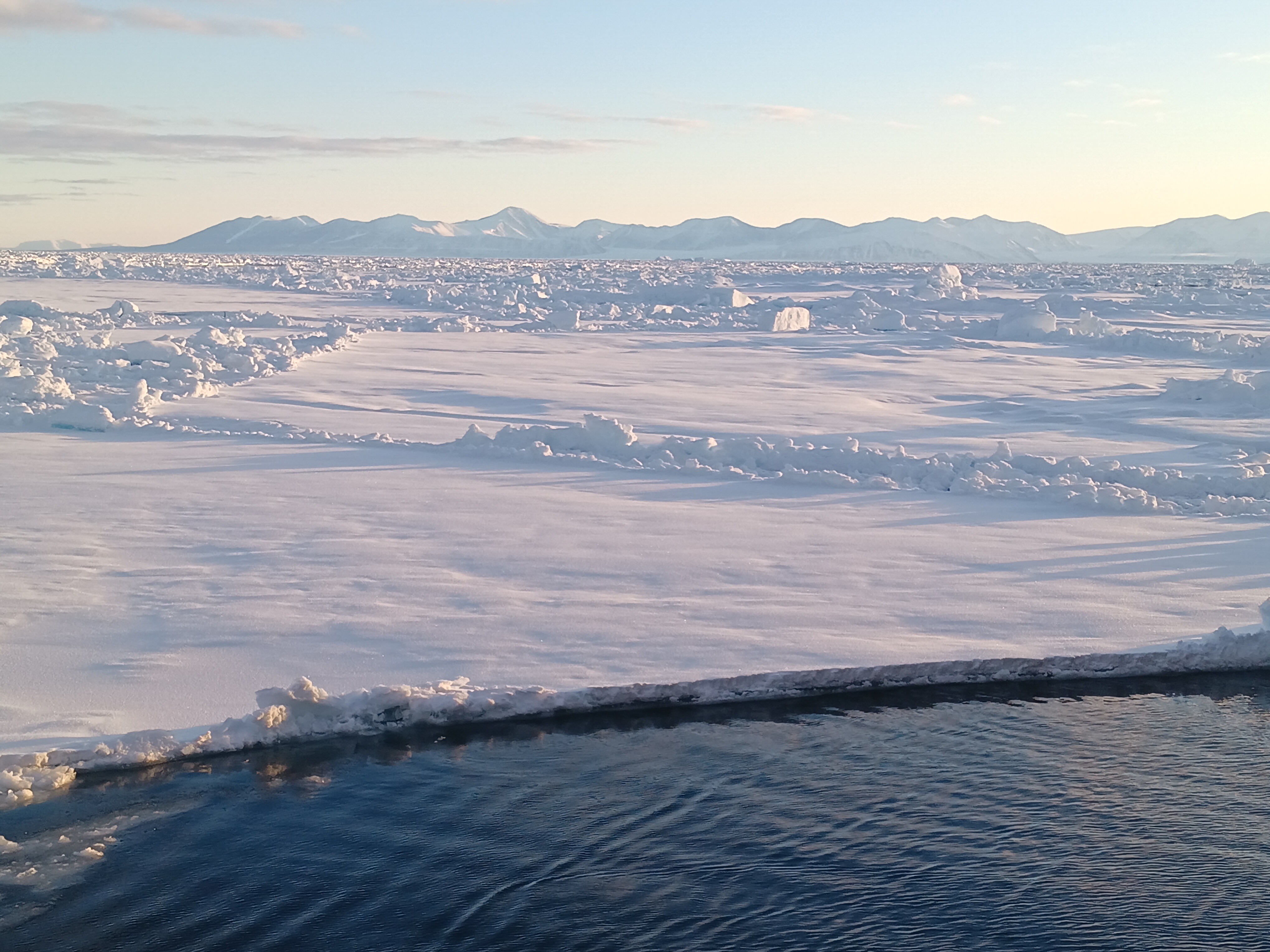
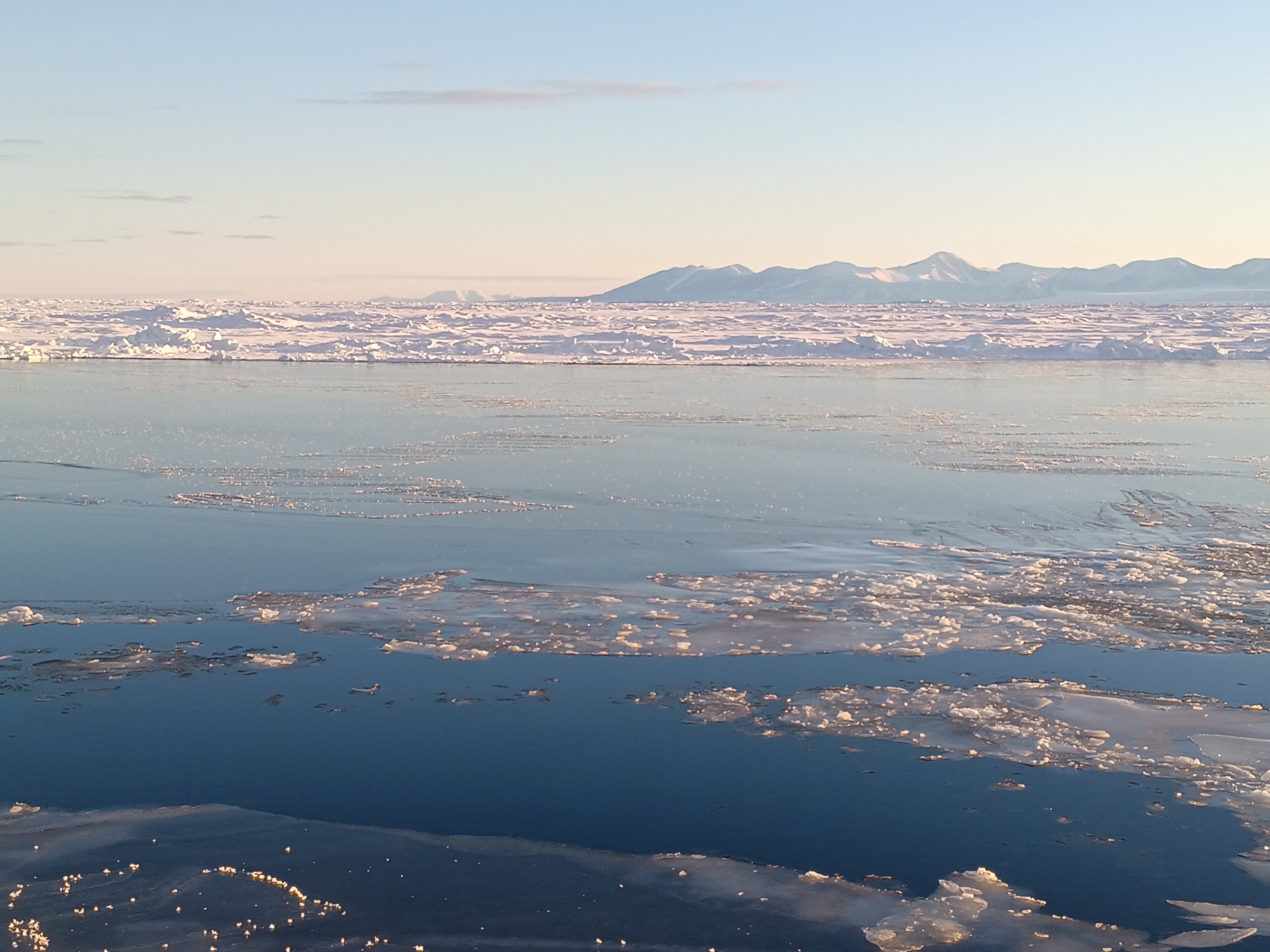
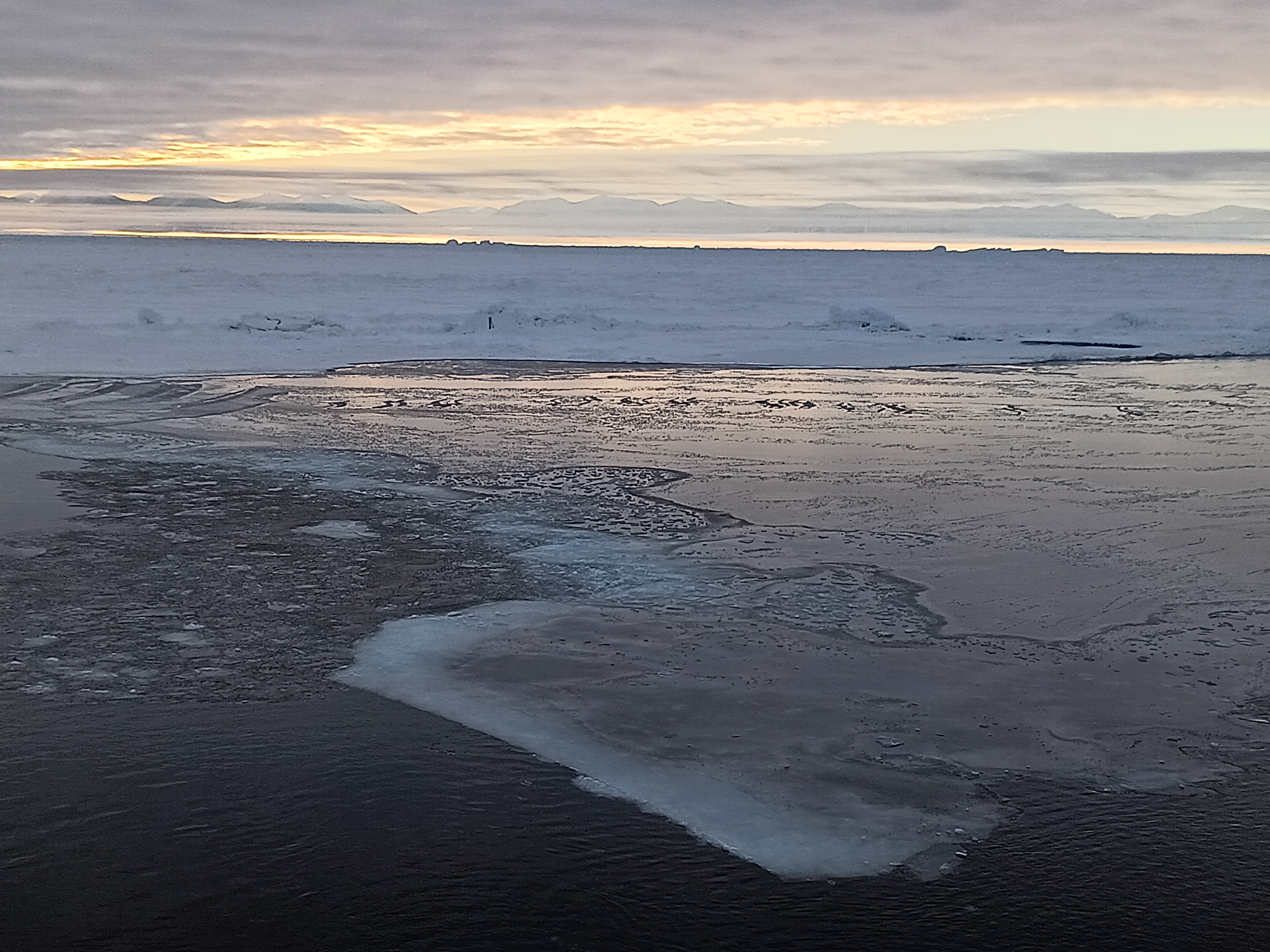
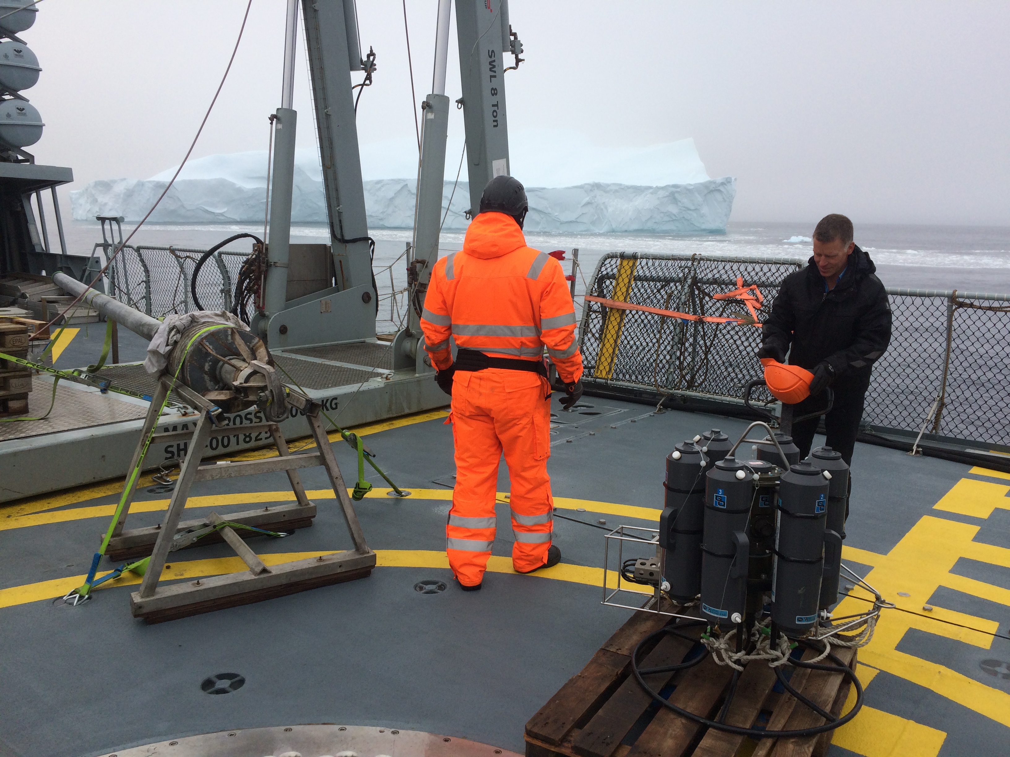
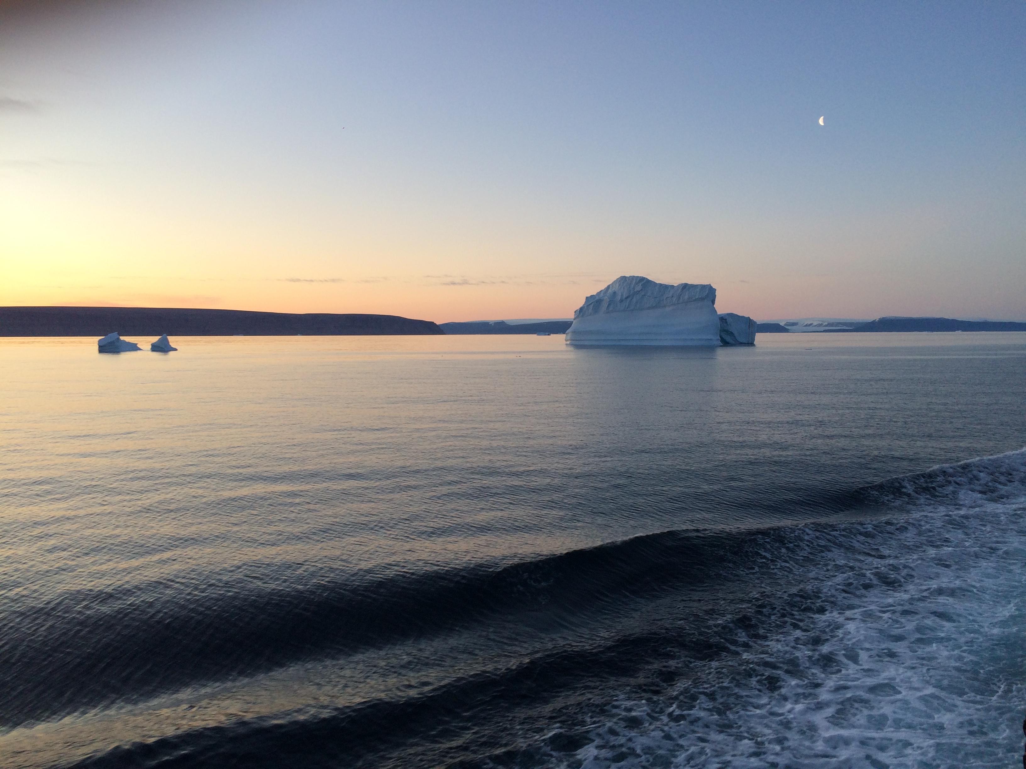
There is so much more to this story as well as additional stories, notice the red dots in the top-left panel between 150-m and 300-m depth that indicate a strong flow to the south and east, but I save this for later. I also do not wish to tell you about the two ocean sensors we quickly deployed at this location to stay there until we, perhaps, recover them with new data next year or the year there after. I do wish to close this essay, however, with the view of Greenland that we had where we discovered Claudia’s coastal current. Science is fun, exciting, and always surprises.


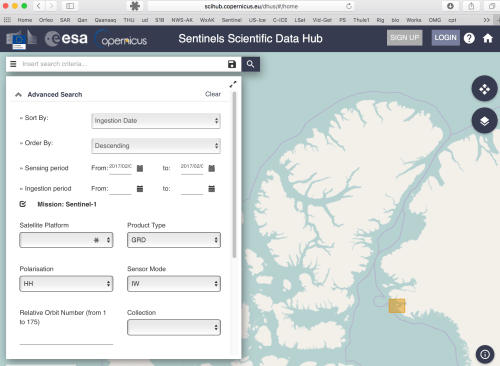
![Screenshot of SNAP software and processing with [1] input and [2] output of the Feb.-5, 2017 data from Wolstenholme Fjord.](https://icyseas.org/wp-content/uploads/2017/02/screen-shot-2017-02-07-at-5-06-35-pm.png?w=500)
![Working the Night shift aboard CCGS Henry Larsen in the CTD van in Aug.-2012. [Photo Credit: Renske Gelderloos]](https://icyseas.org/wp-content/uploads/2014/09/aug_8_ctd_andreas_01.jpg?w=500)
![Polar bear as seen in Kennedy Channel on Aug.-12, 2012. [Photo Credit: Kirk McNeil, Labrador from aboard the Canadian Coast Guard Ship Henry Larsen]](https://icyseas.org/wp-content/uploads/2012/08/polarbear-kirkmcneil_0418.jpg?w=500)
![Icebreaker taking on waves on the stern during a fall storm in the Beaufort Sea in October 2004. [Photo Credit: Chris Linder, Woods Hole Oceanographic Institution]](https://icyseas.org/wp-content/uploads/2016/06/picture1.png)

