Tag Archives: polynya

Greenland Oceanography by Sled and Snowmobile

Wind chill matters in Greenland because one must see and breath. This implies exposed skin that will hurt and sting at first. Ignoring this sting for a few minutes, I notice that the pain goes away, because the flesh has frozen which kills nerves and skin tissue. The problem becomes worse as one drives by snowmobile to work on the sea ice which I do these days almost every day.

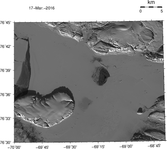
Navigating on the sea ice by identifying ice bergs with LandSat imagery. The imagery also shows polynyas and thin ice in the area. [Photo Credit: Sonny Jacobsen]

Mar.-22, 2017 LandSat image of study area with Thule Air Base near bottom right, Saunders Island in the center. Large red dots are stations A, B, and C with Camp-B containing weather station, shelter, and first ocean mooring. My PhD student Pat Ryan prepared this at the University of Delaware.

My companion on the ice is Sonny Jacobsen who knows and reads the land, ice, and everything living on and below it. He teaches me how to drive the snowmobile, how to watch for tracks in the snow, how to pack a sled, and demonstrates ingenuity to apply tools and materials on-hand to fix a problem good enough to get home and devise a new and better way to get a challenging task done. Here he is designing and rigging what is to become our “Research Sled” R/S Peter Freuchen, but I am a little ahead of my story:

Sonny Jacobsen on Mar.-27, 2017 on Thule Air Base building a self-contained sled for ocean profiling.

First we set up a shelter in the center of what will hopefully soon become an array of ocean sensors and acoustic modems to move data wirelessly through the water from point A in the north-west via point B to point C. Point C will become the pier at Thule Air Base while the tent is at B that I call Camp-B:

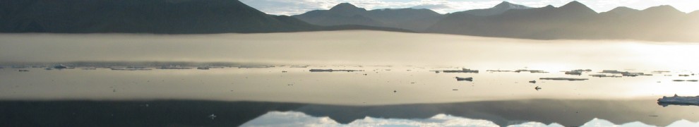
Ice Fishing shelter to the north-east of Saunders Island seen to the left in the background.

Next, we set up an automated weather station (AWS) next to this site, because winds and temperatures on land next to hills, glaciers, and ice sheets are not always the same 10 or 20 km offshore in the fjord. It is a risk-mitigating safety factor to know the weather in the study area BEFORE driving there for 30-60 minutes to spend the day out on the ice. It does not hurt, that this AWS is also collecting most useful scientific data, but again, I am slightly ahead of my story:

Weather station with shelter at Camp-B with the northern shores of Wolstenholme Fjord in the background. Iridium antenna appears just above the iceberg on the sidebar of the station. Winds are measured at 3.2 m above the ground.

With shelter and weather station established and working well, we decided to drill a 10” hole through 0.6 m thin ice to deploy a string of ocean instruments from just below the ice bottom to the sea floor 110 m below. Preparing for this all friday (Mar.-24), we deploy 22 sensors on a kevlar line of which 20 record internally and must be recovered while 2 connect via cables to the weather station to report ocean temperature and salinity along with winds and air temperatures. It feels a little like building with pieces of Lego as I did as a kid. Engineers and scientists, perhaps, are trained early in this sort of thing.

Weather station with ocean mooring (bottom right) attached with eastern Saunders Island in the background on Sunday Mar.-26, 2017.

Sadly, only the ocean sensor at the surface works while the one at the bottom does not talk to me. I can only suspect that I bend a pin on the connector trying to connect very stiff rubber sealing copper pins from the cable with terminations equally stiff in the cold, however, there are other ways to get at the bottom properties albeit with a lot more effort … which brings me to R/S Peter Freuchen shown here during its maiden voyage yesterday:

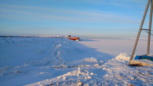
R/S Peter Freuchen in front of 10” hole (bottom right) for deployment of a profiling ocean sensor. The long pipes looking like an A-frame on a ship become a tripod centered over the hole with the electrical winch to drive rope and with sensors (not shown) over a block into the ocean. This was yesterday Mar.-28, 2017 on the way from Camp-B back to Thule Air Base.

The trial of this research sled was successful, however, as all good trials, it revealed several weaknesses and unanticipated problems that all have solutions that we will make today and tomorrow. The design has to be simple to be workable in -25 C with some wind and we will strip away layers of complexities that are “nice to have” but not essential such as a line counter and the speed at which the line goes into the water. There can not be too many cables or lines or attachments, because any exposure to the elements becomes hard labor. This becomes challenging with any gear leaving the ocean (rope, sensors) and splattering water on other components. Recall that ocean water is VERY hot at -1.7 C relative to -25 C air temperatures. This means that ANYTHING from the ocean will freezes instantly when in contact with air. Efficiency and economy matter … as does body heat to keep critical sensors and batteries warm.

A big Thank-You to Operation IceBridge’s John Woods for something related to this post that I wish not to advertise 😉

Preparing Ocean Work outside Thule Air Base

I am heading to North Greenland in 3 days time to work where temperatures will be close to -20 F. The ocean is covered by 3-4 feet of sea ice that is frozen to land. We will drill lots of ice holes to deploy ocean sensors that will connect via cables to weather stations and satellite phone. Fancy $20,000 GPS units will measure the tides across the fjord and provide a group of future Naval officers a reference for their fancy electronic gear to measure sea ice thickness remotely by walking and comparing results to those obtained from planes overhead. Cool and cold fun.

img_20170302_111051404

The ocean pier at Thule Air Base in Greenland in March 2017. The view is towards the north-west along my proposed mooring line [Photo Credit: Sean Baker]

There has been much packing and shipping the last weeks, about 2300 lbs to be precise,which made my body stiff and sore. Another way to hurt my aging body was to learn shotgun shooting for the unlikely polar bear encounter on the sea ice. My shoulder still hurts from the recoil blasts of the 12 gauge pump-action gun with 3” long cartridges that included a 1 oz. lead slug. I also tested a cot and sleeping bag that will be with me on the ice for emergencies. The night in my garden a few days ago was cozy, but the cot required an insulation mattress, as it was too close to the ground. It was rough sleeping, because of unexpected noises not cold, but I did sleep some and woke up when the sun came up.

Cot, air mattress, and down sleeping bag testing in my garden after a rough night.

Cot, air mattress, and down sleeping bag testing in my garden after a rough night.

The clear skies over Thule during the 2 weeks that the sun is up again also gave me the first Landsat image. It shows the landfast sea ice, but it also shows its very limited extend as very thin ice and perhaps even open water occurs while the winds blow along the coast from the north. This cold wind moves the mobile sea ice offshore to the west thus opening up the oceans that will promptly freeze, however, the back ocean still shows under the inch-thin new ice:

Wolstenholme Fjord as seen by LandSat on Feb.-27, 2017. The line with the red dots extends from Thule pier seaward towards the north-west. Note the dark spot near the left-top corner that shows thin new ice or even open water. White contours are ocean depths in meters.

Wolstenholme Fjord as seen by LandSat on Feb.-27, 2017. The line with the red dots extends from Thule pier seaward towards the north-west. Note the dark spot near the left-top corner that shows thin new ice or even open water. White contours are ocean depths in meters.

This thin new ice is the limit of where I expect to be working. After measuring ice thickness directly via drilling through the ice, my first measurement will be that of how temperature and salinity varies from under the ice to the bottom of the ocean.

Working on the sea ice off northern Greenland [Photo credit, Steffen Olsen]

Working on the sea ice off northern Greenland [Photo credit, Steffen Olsen]

Danish friends do this routinely about 60 miles to the north where they work out of the Inughuit community of Qaanaaq, but Inglefield Fjord is much deeper and connects to warm Atlantic waters from the south that, I believe, we do not have in Wolstenholme Fjord. Hence I expect much less heat inside Wolstenholme Fjord and perhaps a different response of three glaciers to ocean forcing. This theory does not help me much as I will have to lower instruments via rope and a winch into the water. How to attach rope to instruments and winch? Knots.

I am very poor at making knots as my hand-eye co-ordination and memory is poor. So I spent some time this week to learn about knots such as

that should work on my braided Kevlar lines that I connect to shackles

Fancy knots on shackles in my home office ... yes, Peter Freuchen is on the bookshelf, too.

Fancy knots on shackles in my home office … yes, Peter Freuchen is on the bookshelf, too.

There are always devils in the many details of field work. Another worry is that my 10” ice-drill is powered by 1 lbs bottles of propane. It is not possible to send these camping propane canisters via air, but larger 20 lbs tanks exist in Thule for grill cooking at the NSF dormitory where I will be staying. So I also will have to learn how to fill the smaller container from the large one. Just ordered another adaptor from Amazon to travel with me on my body to do this.

I am both terribly nervous and excited about the next 6 weeks. This is my first time working on the ice, because before I have always been on icebreakers in summer. These past Arctic summer expeditions on ships created an unreal and distant connection that, I hope, will be shattered by this spring. I will get closer to the cold and icy seas that are my passion. Oceanography by walking on water … ice.

Sea Ice from Satellite at 20-m Resolution

I am a self-taught amateur on remote sensing, but it tickled my pride when a friend at NASA asked me, if I could tell a friend of his at NOAA on how I got my hands on data to produce maps of radar backscatter to describe how the sea ice near Thule Air Base, Greenland changes in time and space.

Wolstenholme Fjord, Greenland Feb.-5, 2017 from Sentinel-1 radar. The data are at 20-m resolution

Wolstenholme Fjord, Greenland Feb.-5, 2017 from Sentinel-1 radar. The data are at 20-m resolution

In about 4 weeks from today I will be working along a line near the red dots A, B, and C which are tentative locations to place ocean sensors below the sea ice after drilling through it with ice fishing gear. The colored line is the bottom depth as it was measured by the USCG Healy in 2003 when I was in Thule for the first time. Faint bottom contours are shown in gray.

I discovered the 20-m Sentinel-1 SAR-C data only 3 weeks ago. They are accessible to me (after making an account) via

https://scihub.copernicus.eu/dhus/#/home

where I then search for a specific geographic area and time frame using the following “product”

Product Type: GRD
Sensor Mode: IW
Polarization: HH

Screenshot on how I search for the Sentinel-1 SAR-C DATA.

Screenshot on how I search for the Sentinel-1 SAR-C DATA.

The more technical detail can be found at

https://sentinel.esa.int/web/sentinel/user-guides/sentinel-1-sar

where one also finds wonderful instructional videos on how to work the software.

The data file(s) for a typical scene are usually ~800 MB, however, for processing I use the free SNAP software (provided by European Space Agency) via a sequence of steps that result in a geotiff file of about 7 MB.

Screenshot of SNAP software and processing with [1] input and [2] output of the Feb.-5, 2017 data from Wolstenholme Fjord.

Screenshot of SNAP software and processing with [1] input and [2] output of the Feb.-5, 2017 data from Wolstenholme Fjord.

This .tiff file I then read with Fortran codes to tailor my own (quantitative or analyses) purposes.

Start of Fortran code to covert the SNAP output geotiff file into an ascii file with latitude, longitude, and backscatter as columns. The code has 143 lines plus 80 lines of comment.

Start of Fortran code to covert the SNAP output geotiff file into an ascii file with latitude, longitude, and backscatter as columns. The code has 143lines plus 80 lines of comment.

The final mapping is done with GMT – General Mapping Tools which I use for almost all my scientific graphing, mapping, and publications.

Please note that I am neither a remote sensing nor a sea-ice expert, but consider myself an observational physical oceanographer who loves his Unix on a MacBook Pro.

Working the Night shift aboard CCGS Henry Larsen in the CTD van in Aug.-2012. [Photo Credit: Renske Gelderloos]

Working the Night shift aboard CCGS Henry Larsen in the CTD van in Aug.-2012. [Photo Credit: Renske Gelderloos]

If only my next problem, working in polar bear country with guns for protection, had as easy a solution.

Polar bear as seen in Kennedy Channel on Aug.-12, 2012. [Photo Credit: Kirk McNeil, Labrador from aboard the Canadian Coast Guard Ship Henry Larsen]

Polar bear as seen in Kennedy Channel on Aug.-12, 2012. [Photo Credit: Kirk McNeil, Labrador from aboard the Canadian Coast Guard Ship Henry Larsen]

Thule, Greenland in Sharp Focus

I want to fly like an eagle
To the sea
Fly like an eagle
Let my spirit carry me

Steve Miller Band, 1976

The eagle “sees” the ground, because the twinkling sensation of light tickles her nerves. Today’s cameras work without the twinkle and tickle. They store numbers (digits) that approximate the amount of light passing through the lens. Satellite sensors work the same way. The data they beam to earth give me the soaring feeling of flying like an eagle, but there is more to the bits and bytes and digits sent home from space to our iPhones, laptops, and the internet.

Aerial photo taken Oct.-13, 1860 of Boston, MA by J.W. Black.

Aerial photo taken Oct.-13, 1860 Boston, MA from a balloon by J.W. Black.

The Metropolitan Museum of Art in New York houses the earliest existing aerial photo that was taken from a balloon hovering 600 meters above Boston, Massachusetts. Within a year the American Civil War broke out and this new technology became an experimental tool of war. It advanced rapidly, when air craft replaced the balloon during the First World War. Sharp photos of bombed-out battle and killing fields along the entire Western Front in France were taken by both Allied and German soldiers every day. Placing these photos on a map for efficient analyses of how a land- sea- or ice-scape changes over time, however, was impossible, because photos do not record precise locations.

Modern satellite photos are different. We now have fancy radar beams, computers, and several Global Position Systems (GPS) with atomic clocks to instantly calculation satellite tracks every second. This is why we now can both take photos from space AND map every dot or pixel that is sensed by the satellite moving overhead at 17,000 miles an hour snapping pictures from 430 miles above. The camera is so good that it resolves the ground at about 45 feet (15 meters). This is what such a (LandSat) picture looks like

LandSat photo/map of Thule, Greenland Mar.-17, 2016. The airfield of Thule Air Force Base is seen near the bottom on the right. The island in ice-covered Westenholme Fjord is Saunders Island (bottom left) while the glacier top right is Chamberlin Gletscher.

LandSat photo/map of Thule, Greenland Mar.-17, 2016. The airfield of Thule Air Force Base is seen near the bottom on the right. The island in ice-covered Westenholme Fjord is Saunders Island (bottom left) while the glacier top right is Chamberlin Gletscher.

Everyone can download these photos from the United States Geological Survey which maintains a wonderful photo and data collection archive at

http://earthexplorer.usgs.gov

but the tricky part is to turn these images or photos into maps which I have done here. More specifically, I wrote a set of c-shell and nawk scripts along with Fortran programs on my laptop to attach to each number for the light sensed by the satellite (the photo) another two numbers (the map). These are latitude and longitude that uniquely fix a location on the earth’s surface. A “normal” photo today has a few “Mega-Pixels,” that is, a few million dots. Each scene of LandSat, however, has about 324 million dots. This is why you can discern both the runways of Thule Air Force Base at 68 degrees 45′ West longitude and 76 degrees 32′ North latitude. The pier into the ice-covered ocean is just a tad to the south of Dundas Mountain at 68:54′ W and 76:34′ N. A scale of 5 kilometers is shown at the top on the right. For spatial context, here is a photo of the pier with the mountain in the background, that is, the object shown in the photo such as mountain, ship, and Helen serves a rough, but imprecise reference:

Dr. Helen Johnson in August 2009 on the pier of Thule AFB with CCGS Henry Larsen and Dundas Mountain in the background. [Credit: Andreas Muenchow]

Dr. Helen Johnson in August 2009 on the pier of Thule AFB with CCGS Henry Larsen and Dundas Mountain in the background. [Credit: Andreas Muenchow]

This photo shows the airfield and Saunders Island

Thule AFB with its airport, pier, and ice-covered ocean in the summer. The island is Saunders Island. The ship is most likely the CCGS Henry Larsen in 2007. [Credit: Unknown]

Thule AFB with its airport, pier, and ice-covered ocean in the summer. The island is Saunders Island. The ship is most likely the CCGS Henry Larsen in 2007. [Credit: Unknown]

The satellite image of the ice-covered fjord with Thule, Saunders Island, and Chamberlin Gletschers shows a richly texture field of sea ice. The sea ice is stuck to land and not moving except in the west (top left) where it starts to break up as seen by the dark gray piece that shows ‘black’ water peeking from below a very thin layer of new ice. There is also a polynya at 69:15′ W and 76:39′ N just to the south of an island off a cape. A polynya is open water that shows as black of very dark patches. A similar albeit weaker feature also shows to the east of Saunders Island, but it is frozen over, but the ice there is not as thick as it is over the rest of Westenholme Fjord. I suspect that larger tidal currents over shallow water mix ocean heat up to the surface to keep these waters covered by water or dangerously thin ice. There are also many icebergs grounded in the fjord. They cast shadows and from the length of these shadows one could estimate their height. Here is another such photo from 2 days ago:

LandSat photo/map of Thule, Greenland Mar.-21, 2016. The airfield of Thule Air Force Base is seen near the bottom on the right. The island in ice-covered Westenholme Fjord is Saunders Island (bottom left) while the glacier top right is Chamberlin Gletscher.

LandSat photo/map of Thule, Greenland Mar.-21, 2016. The airfield of Thule Air Force Base is seen near the bottom on the right. The island in ice-covered Westenholme Fjord is Saunders Island (bottom left) while the glacier top right is Chamberlin Gletscher.

I am using the satellite data and maps here to plan an experiment on the sea ice of Westenholme Fjord. Next year in March/April I will lead a team of oceanographers, engineers, and acousticians to place and test an underwater network to send data from the bottom of the ocean under the sea ice near Saunders Island to the pier at Thule and from there on to the internet. We plan to whisper from one underwater listening post to another to communicate over long ranges (20-50 kilometers) via a network of relay stations each operating smartly at very low energy levels. We will deploy these stations through holes drilled through the landfast ice 1-2 meters thick. The work is very exploratory and is funded by the National Science Foundation. Wish us luck, as we can and will use it … along with aerial photography that we turn into maps.

Sun Set in Nares Strait, Greenland

The sun bathed the southern reaches of Nares Strait in light again after four months of total darkness of the polar night. It is still cold, about -30 degrees centigrade, but the long shadows cast by mountains, hills, and even icebergs from Humbold Glacier are a feast for my eyes:

Kane Basin with Humbold Glacier, Greenland in the east, Ellesmere Island, Canada in the west as well as Smith Sound in the south, and Kennedy Channel of Nares Strait in the north. The visible image was taken Mar.-2, 2015 at 17:30 UTC by MODIS Terra.

Kane Basin with Humbold Glacier, Greenland in the east, Ellesmere Island, Canada in the west as well as Smith Sound in the south, and Kennedy Channel of Nares Strait in the north. The visible image was taken Mar.-2, 2015 at 17:30 UTC by MODIS Terra.

The sun dipped above the southern horizon just for a few hours. The light reflected by the ice and snow of North Greenland was captured by a satellite overhead. From these data I constructed the above image with the axes in km. The frame is big enough to fit both Denmark and Massachusetts into it. The image shows the southern entrance to Nares Strait with its prominent ice arch and the “North Water” polynya in the south. You can “see” individual ice floes in this image as well as rows of sea smoke over the thin ice of the polynya that are all resolved at the 250-m pixel size. Petermann is still dark and not shown, but give it a week, and we’ll get sun there also.

I will be watching this ice arch closely, because together with a group of 50 international scientists I am scheduled to sail these icy waters aboard the Swedish icebreaker Oden this summer for a multitude of experiments to take place in Petermann Fjord with data sampling of adjacent ice, ocean, and land. As a group we will try to reconstruct climate and its physical processes that impact change from tidal to glacial cycles.