Category Archives: Arctic Glacier

Greenland Glacier-Driven Ocean Circulation

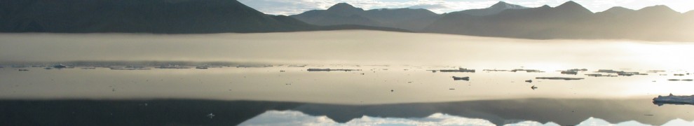
Greenland’s coastal glaciers melt, shrink, and add to globally rising sealevel. They also drive local ocean currents that move icebergs around unless they are stuck on the bottom. The glaciers’ melt is cold fresh water while the adjacent ocean is both salty and warm. Checking on what we may expect against observations, I here use data from NASA’s Ocean Melts Greenland initiative that dropped ocean probes from an airplane into the ice waters off coastal Greenland to measure ocean temperature and salinity.

For six years these data show how the coastal ocean off Greenland varies from location to location next to glaciers as well as from year to year. More specifically, I picked Melville Bay in North-West Greenland for both its many glaciers and many dropped NASA ocean sensors. The ocean data allow me to estimate ocean currents by using a 100 year old physics method. I just taught this to a small class of undergraduate science students at the University of Delaware. My students are strong in biology, but weak on ocean physics. This essay is for them.

Melville Bay is a coastal area off north-west Greenland between the town of Upernavik (Kalaallisut in Greenlandic) near 73 N latitude where 1100 people live and the village of Savissivik (Havighivik in Inuktun) at 76 N latitude where 60 Inuit live. There are no other towns or settlements between these two villages that are about as far apart as Boston is from Philadelphia, PA. Imagine there were no roads from Boston to New York to Philadelphia but only one large glacier next to another large glacier. This is Melville Bay.

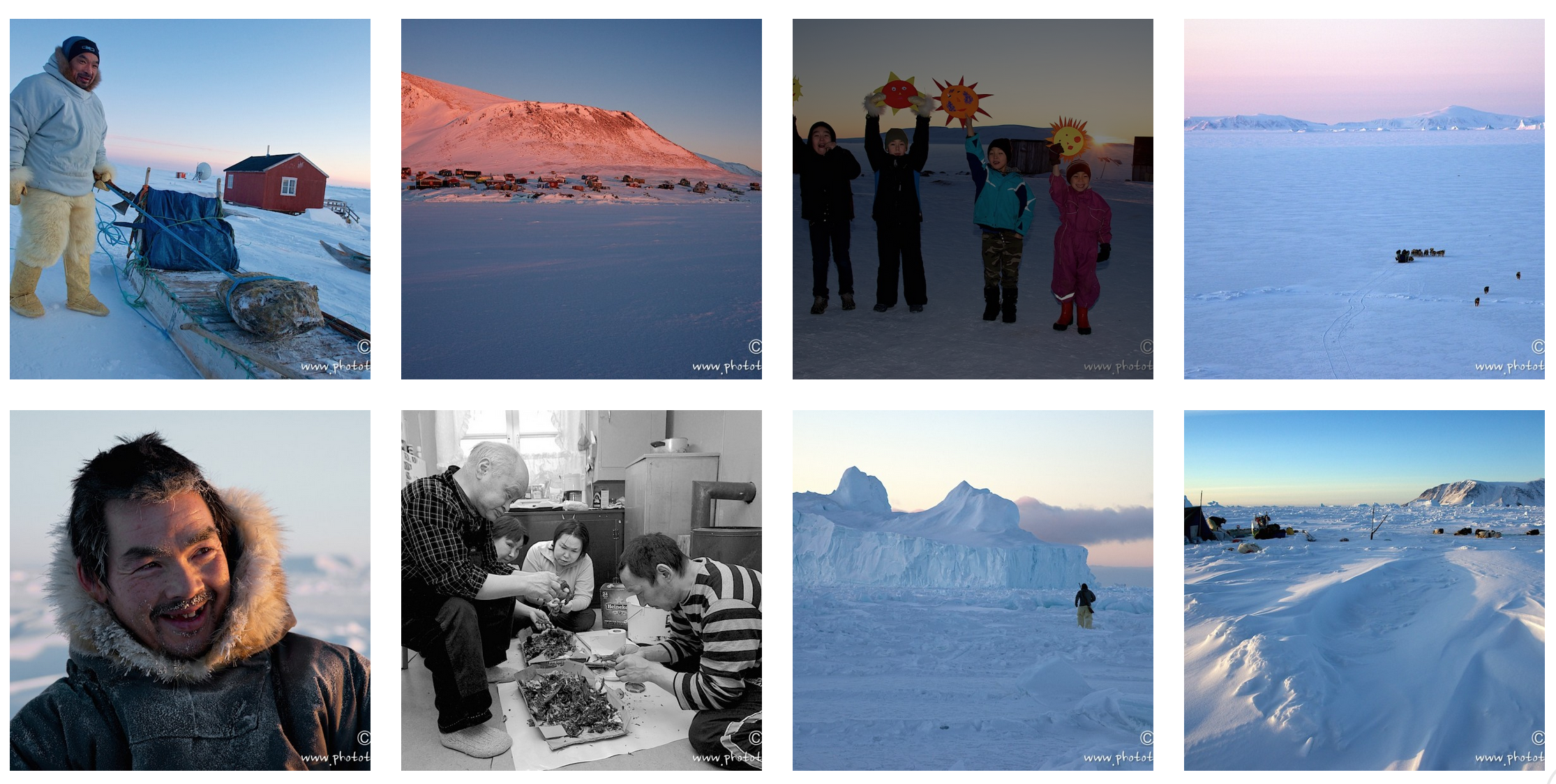
Below I show an excellent set of photos of Savissivik by a French husband and wife team who visited in 2013/14. Their photographic gallery captures elements of contemporary subsistence living in remote Greenland where animals like seals, birds, fish, narwhal, and polar bears provide food, fuel, clothing, and income.

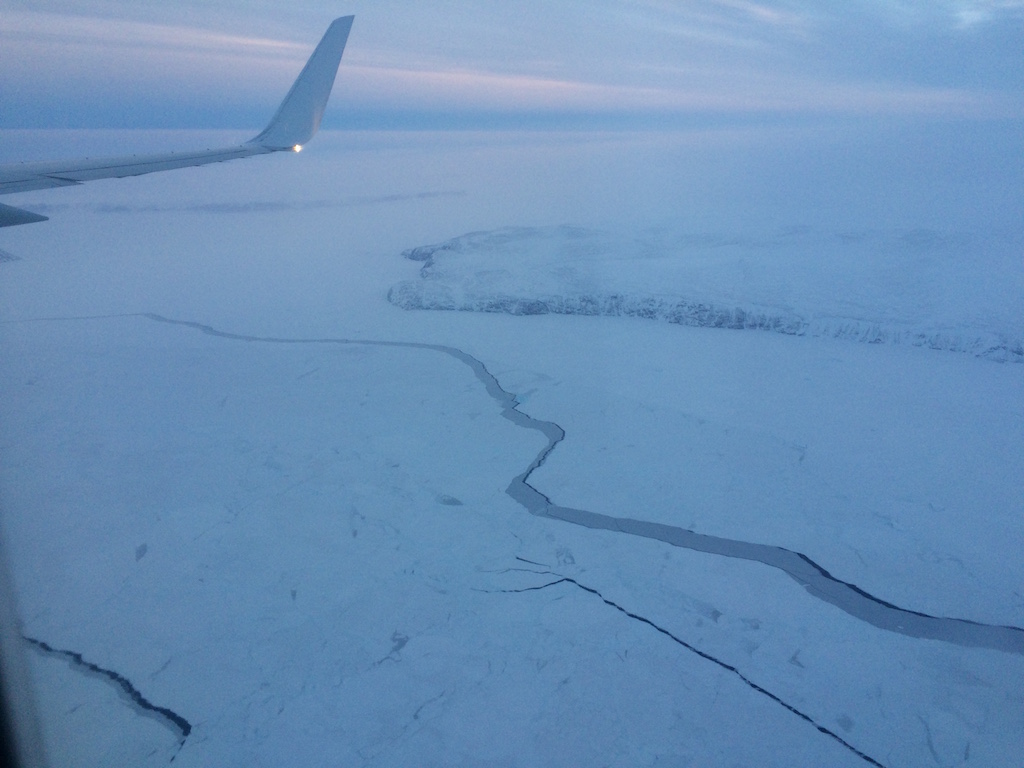
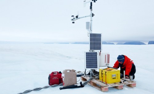
NASA dropped some 50 ocean sensors into Melville Bay froma plane during the short summer seasons each year 2016 through 2021. I met NASA pilots, engineers, and scientists doing their experiments when I was doing mine from a snowmobile in April of 2017 and again with Danish friends from a Navy ship in August of 2021, but these are stories for another day.

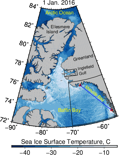
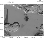
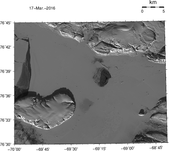
Let me start with a map of where NASA dropped their ocean profiling floats into Melville Bay and thus introduce the data. While the surface waters are usually near the freezing point, waters 300-400 meters deep down are much warmer. They originate from the Atlantic Ocean to the south and one of the goals of NASA’s “Ocean Melts Greenland” campaigns was to determine if and how these Atlantic waters reach the coastal glaciers. Most glaciers of Melville extend into this warm ocean layer and thus are melted by the ocean.

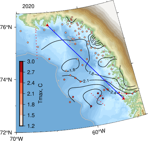
In the map above I paint the maximal temperatures in red and the bottom depths in blue tones. The profile on the right shows data for all depths at one station. As salinity increases uniformly (red curve) the temperature increases to a maximum near 300-m depth (black curve). It is this maximal subsurface temperature that I extract for each station and then put on the contour and station map on the left. The straight blue line connects Upernavik in the south with Sassivik in the north. It is an arbitrary line, coast-to-coast cutting across Melville Bay.

The warmest warm waters we find near Upernavik in the south and within a broad submarine canyon that brings even warmer waters from Baffin Bay towards the coast. Temperatures here exceed 2.4 or even 2.7 degrees Celsius. Most coastal waters along Melville Bay have a temperature maximum of about 1.5 to 1.8 degrees Celcius (about 35 Fahrenheit) and this “warm Atlantic” ocean water melts the coastal glaciers. The ocean melts the glaciers summer and winter while the warm air melts it only in summer.

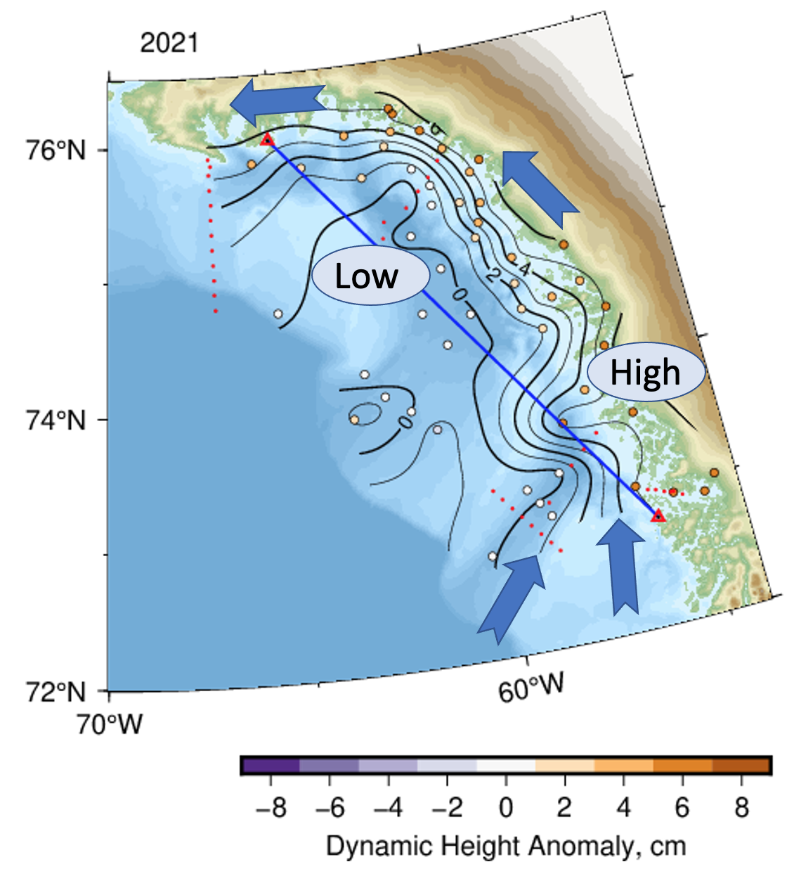
There is more, because the glaciers’ melt also discharge fresh water into the ocean where it mixes to to form a layer of less dense or buoyant water. The buoyant waters create a local sealevel that is a little higher along the coast than farther offshore. The map above indicates that this “little higher sealevel” comes to about 4 cm or 2 inches. If this pressure difference across the shore is balanced by the Coriolis force, as it often does, then an along-shore coastal current results. This coastal current would move all icebergs from south to north unless they get stuck on the bottom. Along the northern coastline of Melville Bay the surface flow is from east to west. The coastal current is strongest near Savissivik where we find a (geostrophic) surface current larger than 40 cm/s. At that speed an iceberg would move more than 21 miles per day. Such strong surface flows are exceptional and diminish rapidly with depth. Hence a freely floating iceberg with a draft of several hundred meters would move much slower than the surface current.

I met a hunter from Savissivik in April of 2017 and for a fast-moving night we discussed the state of local fishing, hunting, living, traveling, and working on the sea ice next to the glaciers of Melville Bay. He invited me to become his apprentice. As such I would now ask him about the surface currents outside his home. Which way does he observe the icebergs to move in summer or winter? Has hunting on the sea ice in winter changed over his life time? When is it safe to travel there with a dog-sled? Could he and I perhaps work together during the spring to deploy ocean sensors through the sea ice? I am dreaming again …
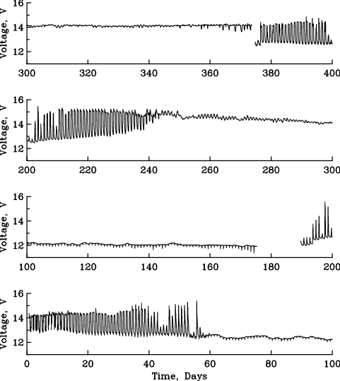
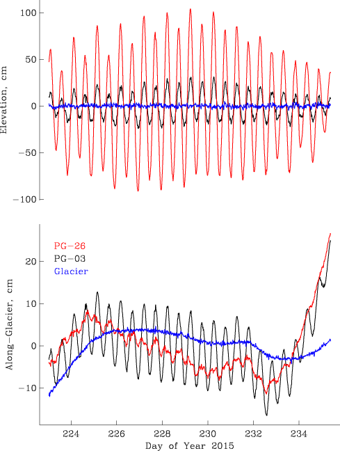
Petermann Gletscher and Greenland Climate Change

Multi-media story of two old-style scientists on a Greenland data rescue mission. Keith (Nicholls) and I were joined by Chris Mooney and Whitney Shefte of the Washington Post who just posted

Testifying before the US Congress back in 2010, I refused to endorse the view that a first large calving at Petermann Gletscher in North Greenland was caused by global warming. Additional events and analyses of new data and old data, however, convinced me that climate change forces Petermann Gletscher into a new and unknown state.

Oceanography below Petermann Gletscher for 400 Days

Ocean data from 810 meters below sea level under one of Greenland’s last remaining ice shelves arrives every 3 hours at my laptop via a 3-conductor copper cable that passes through 100 meter thick ice to connect to a weather station that via a satellite phone system connects to the rest of the world. This Ocean-Weather station on the floating section of Petermann Gletscher has reported for 400 days today. I am still amazed, stunned, and in awe that this works.

The station started 20th August of 2015 as a small part of a larger joint US-Swedish expedition to North Greenland after friends at the British Antarctic Survey drilled holes through the Empire-State-Building thick ice shelf. It is powered by two 12 Volt car batteries that are recharged by two solar panels. When the sun is down, the car batteries run the station as in winter when temperatures reached -46 C. When the sun is up, the solar cells run the station and top off the batteries. The voltage during the last 400 days shows the “health” of the station:

Battery voltage at the Petermann Ocean-Weather Station from Aug.-20, 2015 through  Sept.-23, 2016. The polar night is indicated by slowly declining voltage near 12 V while during the polar day voltage is near 14 V with oscillations in spring and fall during the transition from 24 hours of darkness to 24 hours of sun light.

Battery voltage at the Petermann Ocean-Weather Station from Aug.-20, 2015 through Sept.-23, 2016. The polar night is indicated by slowly declining voltage near 12 V while during the polar day voltage is near 14 V with oscillations in spring and fall during the transition from 24 hours of darkness to 24 hours of sun light.

There is an unexplained outage without data from February 12-25 (Day 175-189) which happened a day after the first data logger shut down completely without ever recovering. Our station has 2 data loggers: A primary unit controls 2 ocean sensors, atmospheric sensors, and the Iridium satellite communication. The secondary unit controls 3 ocean sensors and the GPS that records the moving glacier. Remote access to the secondary logger is via the primary, however, each logger has its own processors, computer code, and back-up memory card.

Inside of University of Delaware command and control of five ocean sensors and surface weather station. Two data loggers are stacked above each other on the left.

Inside of University of Delaware command and control of five ocean sensors and surface weather station. Two data loggers are stacked above each other on the left.

The primary logger failed 11th February 2016 when we received our last data via Iridium satellites until Keith Nicholls and I visited the station 27th and 28th August 2016 via helicopter from Thule, Greenland. Since I could not figure out what went wrong sitting on the ice with the helicopter waiting, I spent a long night without sleep to swap the data logger with a new and tested unit. I rewired sensors to new data logger, switched the Iridium modem, transceiver, and antenna, changed the two car batteries, and now both data loggers with all five ocean sensors have since reported faithfully every 3 hours as scheduled as seen at

http://ows.udel.edu

Lets hope that the station will keep going like as it does now.

The major discovery we made with the ocean data are large and pronounced pulses of fresher and colder melt waters that swosh past our sensors about 5 and 25 meters under the glacier ice. These pulses arrive about every 14 days and this time period provides a clue on what may cause them – tides. A first descriptive report will appear in December in the peer-reviewed journal Oceanography. Our deeper sensors also record increasingly warmer waters, that is, we now see warm (and salty) waters under the glacier that in 2015 we saw more than 100 km to the west in Nares Strait. This suggests that the ocean under the glacier is strongly coupled to the ambient ocean outside the fjord and vice versa. More on this in a separate future posting.

Time series of salinity (top) and potential temperature (bottom) from four ocean sensors deployed under the ice shelf of Petermann Gletscher from 20th of August 2015 through 11th of February 2016. Temperature and salinity scales are inverted to emphasize the vertical arrangements of sensors deployed at 95m (black), 115 (red), 300 m, and 450 m (blue) below sea level. Note the large fortnightly oscillations under the ice shelf at 95 and 115 m depth in the first half of the record. [From Muenchow et al., 2016]

Time series of salinity (top) and potential temperature (bottom) from four ocean sensors deployed under the ice shelf of Petermann Gletscher from 20th of August 2015 through 11th of February 2016. Temperature and salinity scales are inverted in order to emphasize the vertical arrangements of sensors deployed at 95m (black), 115 (red), 300 m, and 450 m (blue) below sea level. Note the large fortnightly oscillations under the ice shelf at 95 and 115 m depth in the first half of the record. [From Muenchow et al., 2016]

P.S.: The installation and year-1 analyses were supported by a grants from NASA and the Jet Propulsion Laboratory, respectively, while the current work is supported by NSF for the next 3 years. Views and opinions are mine and do not reflect those of the funding agencies.

The Ice Shelf of Petermann Gletscher, North Greenland and its ocean below: Introductions

“In 1921 owing to starvation I had to go directly from Cape Heiberg-Juergensen to our cache at Cape Agassiz … during this journey the greater part of the glacier was mapped.” — Lauge Koch, 1928

Traveling by dog sled, Geologist Lauge Koch mapped Petermann Gletscher in 1921 after he and three Inuit companions crossed it on a journey to explore northern North Greenland. They discovered and named Steensby, Ryder, and H.C. Ostenfeld Glaciers that all had floating ice shelves as does Petermann (Ahnert, 1963; Higgins, 1990). In Figure 1 I reproduce the historic map of Koch (1928) that also contains his track in in 1917 and 1921 both across the terminus and across its upstream ice stream. In 1921 all four starved travelers returned safely after living off the land. Four years earlier, however, they were not so lucky: two traveling companions died on a similar journey in 1917 (Rasmussen, 1923).

Maps of Petermann Gletscher by Lauge Koch from 1917 and 1921 dog sleds and 2015 from MODIS-Terra.

Only 20 years after Lauge Koch’s expeditions by dog sled, air planes and radar arrived in North Greenland with the onset of the Cold War. The Arctic Ocean to the north became a battle space along with its bordering land and ice masses of northern Greenland, Ellesmere Island, Canada, Alaska, and Siberia. Weather stations were established in 1947 at Eureka by aircraft and in 1950 at Alert by US icebreaker to support military aviation (Johnson, 1990). In 1951 more than 12,000 US military men and women descended on a small trading post called Thule that Knud Rasmussen and Peter Freuchen had established 40 years earlier to support their own and Lauge Koch’s dog-sled expeditions across Greenland (Freuchen, 1935). “Operation Blue Jay” built Thule Air Force Base as a forward station for fighter jets, nuclear armed bombers, and early warning radar systems. The radars were to detect ballistic missiles crossing the Arctic Ocean from Eurasia to North America while bombers were to retaliate in case of a nuclear attack from the Soviet Union.

An F-102 jet of the 332d Fighter-Interceptor Squadron at Thule AFB in 1960. [Credit: United States Air Force]

An F-102 jet of the 332d Fighter-Interceptor Squadron at Thule AFB in 1960. [Credit: United States Air Force]

About another 60 years later, the jets, the bombers, and the communist threat were all gone, but the Thule Air Force Base is still there as the gateway to North Greenland. It is also the only deep water port within a 1,000 mile radius where US, Canadian, Danish, and Swedish ships all stop to receive and discharge their crews and scientists. Since 2009 Thule AFB also serves as the northern base for annual Operation IceBridge flights over North Greenland to map the changing ice sheets and glaciers.

The establishment of military weather stations and airfields in the high Arctic coincided with the discovery of massive ice islands drifting freely in the Arctic Ocean. On Aug.-14, 1946 airmen of the 46th Strategic Reconnaissance Squadron of the US Air Force discovered a moving ice islands with an area of about 200 square that was kept secret until Nov.-1950 (Koenig et al, 1950). Most of these ice islands originated from rapidly disintegrating ice shelves to the north of Ellesmere island (Jeffries, 1992; Copland 2007), however, the first historical description of an ice islands from Petermann Gletscher came from Franz Boas in 1883 who established a German station in Cumberland Sound at 65 N latitude and 65 W longitude as part of the first Polar Year.

Petermann Ice Island of 2012 at the entrance of Petermann Fjord. The view is to the north-west with Ellesmere Island, Canada in the background. [Photo Credit: Jonathan Poole, CCGS Henry Larsen]

Petermann Ice Island of 2012 at the entrance of Petermann Fjord. The view is to the north-west with Ellesmere Island, Canada in the background. [Photo Credit: Jonathan Poole, CCGS Henry Larsen]

Without knowing the source of the massive tabular iceberg the German physicist Franz Boas reported detailed measurements of ice thickness, extend, and undulating surface features of an ice island in Cumberland Sound that all match scales and characteristics of Petermann Gletscher (Boas, 1885). These characteristics were first described by Dr. Richard Croppinger, surgeon of a British Naval expedition in 1874/75 (Nares, 1876). Dr. Croppinger identified the terminus of Petermann Gletscher as a floating ice shelf when he noticed vertical tidal motions of the glacier from sextant measurements a fixed point (Nares, 1876). His observations on tides were the last until a group of us deployed 3 fancy GPS units on the glacier last summer.

These fancy GPS receivers give centimeter accuracy vertical motions at 30 second intervals. Here is what the deployment of 3 such units in August of 2015 gives me:

Vertical (top) and horizontal (bottom) motion of Petermann Gletscher from GPS referenced to a GPS base station on bed rock at Kap Schoubye. Note the attenuation of the tide from 26 km sea ward of the grounding line (red) to at the grounding line (black) and 15 km landward of the grounding line (blue). The horizontal location motion has the mean motion removed to emphasize short-term change over the much, much larger forward motion of the glacier that varies from about ~700 (black) to ~1250 meters per year (red).

Vertical (top) and horizontal (bottom) motion of Petermann Gletscher from GPS referenced to a GPS base station on bed rock at Kap Schoubye. Note the attenuation of the tide from 26 km sea ward of the grounding line (red) to at the grounding line (black) and 15 km landward of the grounding line (blue). The horizontal location motion has the mean motion removed to emphasize short-term change over the much, much larger forward motion of the glacier that varies from about ~700 (black) to ~1250 meters per year (red).

We have indeed come a far way during the last 150 years or so. Mapping of remote landscape and icescape by starvation and dog-sled has been replaced by daily satellite imagery. Navigation by sextant and a mechanical clock has been replaced by GPS and atomic clock whose errors are further reduced by a local reference GPS. These fancy units and advanced data processing allow me to tell the vertical difference between the top of my iPhone sitting on a table in my garden from the table.

Working at in the garden at home preparing for field work.

Working at in the garden at home preparing for field work near Petermann Fjord.

P.S.: This is the first in a series of essays that I am currently developing into a peer-reviewed submission to the Oceanography Magazine of the Oceanography Society. The work is funded by NASA and NSF with grants to the University of Delaware.

Ahnert, F. 1963. The terminal disintegration of Steensby Gletscher, North Greenland. Journal of Glaciology 4 (35): 537-545.

Boas, F. 1885. Baffin-Land, geographische Ergebnisse einer in den Jahren 1883 und 1884 ausgeführten Forschungsreise. Petermann’s Mitteilungen Ergänzungsheft 80: 1-100.

Copland, L., D.R. Mueller, and L. Weir. 2007. Rapid loss of the Ayles Ice Shelf, Ellesmere Island, Canada. Geophysical Research Letters 34 (L21501): doi:10.1029/2007GL031809.

Freuchen, P. 1935. Arctic adventures: My life in the frozen North. Farrar & Rinehard, NY, 467 pp.

Higgins, A.K. 1990. North Greenland glacier velocities and calf ice production. Polarforschung 60 (1): 1-23.

Jeffries, M. 1992. Arctic ice shelves and ice islands: Origin, growth, and disintegration, physical characteristics, structural-stratigraphic variability, and dynamics. Reviews of Geophysics 30 (3):245-267.

Johnson, J.P. 1990. The establishment of Alert, N.W.T., Canada. Arctic 43 (1): 21-34.

Koch, L., 1928. Contributions to the glaciology of North Greenland. Meddelelser om Gronland 65: 181-464.

Koenig, L.S., K.R. Greenaway, M. Dunbar, and G. Hattersley-Smith. 1952. Arctic ice islands. Arctic 5: 67-103.

Münchow, A., K.K. Falkner, and H. Melling. 2015. Baffin Island and West Greenland current systems in northern Baffin Bay. Progress in Oceanography 132: 305-317.

Münchow, A., L. Padman, and H.A. Fricker. 2014. Interannual changes of the floating ice shelf of Petermann Gletscher, North Greenland, from 2000 to 2012. Journal of Glaciology 60 (221): doi:10.3189/2014JoG13J135.

Nares, G. 1876. The official report of the recent Arctic expedition. John Murray, London,

Rassmussen, K., 1921: Greenland by the Polar Sea: the Story of the thule Expedition from Melville Bay to Cape Morris Jessup, translated from the Danish by Asta and Rowland Kenney, Frederick A. Stokes, New York, NY, 327 pp.

Thule, Greenland in Sharp Focus

I want to fly like an eagle
To the sea
Fly like an eagle
Let my spirit carry me

Steve Miller Band, 1976

The eagle “sees” the ground, because the twinkling sensation of light tickles her nerves. Today’s cameras work without the twinkle and tickle. They store numbers (digits) that approximate the amount of light passing through the lens. Satellite sensors work the same way. The data they beam to earth give me the soaring feeling of flying like an eagle, but there is more to the bits and bytes and digits sent home from space to our iPhones, laptops, and the internet.

Aerial photo taken Oct.-13, 1860 of Boston, MA by J.W. Black.

Aerial photo taken Oct.-13, 1860 Boston, MA from a balloon by J.W. Black.

The Metropolitan Museum of Art in New York houses the earliest existing aerial photo that was taken from a balloon hovering 600 meters above Boston, Massachusetts. Within a year the American Civil War broke out and this new technology became an experimental tool of war. It advanced rapidly, when air craft replaced the balloon during the First World War. Sharp photos of bombed-out battle and killing fields along the entire Western Front in France were taken by both Allied and German soldiers every day. Placing these photos on a map for efficient analyses of how a land- sea- or ice-scape changes over time, however, was impossible, because photos do not record precise locations.

Modern satellite photos are different. We now have fancy radar beams, computers, and several Global Position Systems (GPS) with atomic clocks to instantly calculation satellite tracks every second. This is why we now can both take photos from space AND map every dot or pixel that is sensed by the satellite moving overhead at 17,000 miles an hour snapping pictures from 430 miles above. The camera is so good that it resolves the ground at about 45 feet (15 meters). This is what such a (LandSat) picture looks like

LandSat photo/map of Thule, Greenland Mar.-17, 2016. The airfield of Thule Air Force Base is seen near the bottom on the right. The island in ice-covered Westenholme Fjord is Saunders Island (bottom left) while the glacier top right is Chamberlin Gletscher.

LandSat photo/map of Thule, Greenland Mar.-17, 2016. The airfield of Thule Air Force Base is seen near the bottom on the right. The island in ice-covered Westenholme Fjord is Saunders Island (bottom left) while the glacier top right is Chamberlin Gletscher.

Everyone can download these photos from the United States Geological Survey which maintains a wonderful photo and data collection archive at

http://earthexplorer.usgs.gov

but the tricky part is to turn these images or photos into maps which I have done here. More specifically, I wrote a set of c-shell and nawk scripts along with Fortran programs on my laptop to attach to each number for the light sensed by the satellite (the photo) another two numbers (the map). These are latitude and longitude that uniquely fix a location on the earth’s surface. A “normal” photo today has a few “Mega-Pixels,” that is, a few million dots. Each scene of LandSat, however, has about 324 million dots. This is why you can discern both the runways of Thule Air Force Base at 68 degrees 45′ West longitude and 76 degrees 32′ North latitude. The pier into the ice-covered ocean is just a tad to the south of Dundas Mountain at 68:54′ W and 76:34′ N. A scale of 5 kilometers is shown at the top on the right. For spatial context, here is a photo of the pier with the mountain in the background, that is, the object shown in the photo such as mountain, ship, and Helen serves a rough, but imprecise reference:

Dr. Helen Johnson in August 2009 on the pier of Thule AFB with CCGS Henry Larsen and Dundas Mountain in the background. [Credit: Andreas Muenchow]

Dr. Helen Johnson in August 2009 on the pier of Thule AFB with CCGS Henry Larsen and Dundas Mountain in the background. [Credit: Andreas Muenchow]

This photo shows the airfield and Saunders Island

Thule AFB with its airport, pier, and ice-covered ocean in the summer. The island is Saunders Island. The ship is most likely the CCGS Henry Larsen in 2007. [Credit: Unknown]

Thule AFB with its airport, pier, and ice-covered ocean in the summer. The island is Saunders Island. The ship is most likely the CCGS Henry Larsen in 2007. [Credit: Unknown]

The satellite image of the ice-covered fjord with Thule, Saunders Island, and Chamberlin Gletschers shows a richly texture field of sea ice. The sea ice is stuck to land and not moving except in the west (top left) where it starts to break up as seen by the dark gray piece that shows ‘black’ water peeking from below a very thin layer of new ice. There is also a polynya at 69:15′ W and 76:39′ N just to the south of an island off a cape. A polynya is open water that shows as black of very dark patches. A similar albeit weaker feature also shows to the east of Saunders Island, but it is frozen over, but the ice there is not as thick as it is over the rest of Westenholme Fjord. I suspect that larger tidal currents over shallow water mix ocean heat up to the surface to keep these waters covered by water or dangerously thin ice. There are also many icebergs grounded in the fjord. They cast shadows and from the length of these shadows one could estimate their height. Here is another such photo from 2 days ago:

LandSat photo/map of Thule, Greenland Mar.-21, 2016. The airfield of Thule Air Force Base is seen near the bottom on the right. The island in ice-covered Westenholme Fjord is Saunders Island (bottom left) while the glacier top right is Chamberlin Gletscher.

LandSat photo/map of Thule, Greenland Mar.-21, 2016. The airfield of Thule Air Force Base is seen near the bottom on the right. The island in ice-covered Westenholme Fjord is Saunders Island (bottom left) while the glacier top right is Chamberlin Gletscher.

I am using the satellite data and maps here to plan an experiment on the sea ice of Westenholme Fjord. Next year in March/April I will lead a team of oceanographers, engineers, and acousticians to place and test an underwater network to send data from the bottom of the ocean under the sea ice near Saunders Island to the pier at Thule and from there on to the internet. We plan to whisper from one underwater listening post to another to communicate over long ranges (20-50 kilometers) via a network of relay stations each operating smartly at very low energy levels. We will deploy these stations through holes drilled through the landfast ice 1-2 meters thick. The work is very exploratory and is funded by the National Science Foundation. Wish us luck, as we can and will use it … along with aerial photography that we turn into maps.