“In 1921 owing to starvation I had to go directly from Cape Heiberg-Juergensen to our cache at Cape Agassiz … during this journey the greater part of the glacier was mapped.” — Lauge Koch, 1928
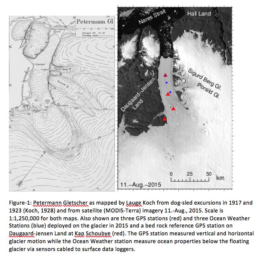
Traveling by dog sled, Geologist Lauge Koch mapped Petermann Gletscher in 1921 after he and three Inuit companions crossed it on a journey to explore northern North Greenland. They discovered and named Steensby, Ryder, and H.C. Ostenfeld Glaciers that all had floating ice shelves as does Petermann (Ahnert, 1963; Higgins, 1990). In Figure 1 I reproduce the historic map of Koch (1928) that also contains his track in in 1917 and 1921 both across the terminus and across its upstream ice stream. In 1921 all four starved travelers returned safely after living off the land. Four years earlier, however, they were not so lucky: two traveling companions died on a similar journey in 1917 (Rasmussen, 1923).

Only 20 years after Lauge Koch’s expeditions by dog sled, air planes and radar arrived in North Greenland with the onset of the Cold War. The Arctic Ocean to the north became a battle space along with its bordering land and ice masses of northern Greenland, Ellesmere Island, Canada, Alaska, and Siberia. Weather stations were established in 1947 at Eureka by aircraft and in 1950 at Alert by US icebreaker to support military aviation (Johnson, 1990). In 1951 more than 12,000 US military men and women descended on a small trading post called Thule that Knud Rasmussen and Peter Freuchen had established 40 years earlier to support their own and Lauge Koch’s dog-sled expeditions across Greenland (Freuchen, 1935). “Operation Blue Jay” built Thule Air Force Base as a forward station for fighter jets, nuclear armed bombers, and early warning radar systems. The radars were to detect ballistic missiles crossing the Arctic Ocean from Eurasia to North America while bombers were to retaliate in case of a nuclear attack from the Soviet Union.
![An F-102 jet of the 332d Fighter-Interceptor Squadron at Thule AFB in 1960. [Credit: United States Air Force]](https://icyseas.org/wp-content/uploads/2013/06/332d_fighter-interceptor_squadron_-_f-102_-_thule_ab.jpg?w=500&h=249)
An F-102 jet of the 332d Fighter-Interceptor Squadron at Thule AFB in 1960. [Credit: United States Air Force]
About another 60 years later, the jets, the bombers, and the communist threat were all gone, but the Thule Air Force Base is still there as the gateway to North Greenland. It is also the only deep water port within a 1,000 mile radius where US, Canadian, Danish, and Swedish ships all stop to receive and discharge their crews and scientists. Since 2009 Thule AFB also serves as the northern base for annual Operation IceBridge flights over North Greenland to map the changing ice sheets and glaciers.
-
-
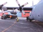
NASA’s Operation IceBridge P3 plane on the tarmac in Thule, Greenland. [Photo Credits: NASA/Icebridge]
-
-
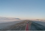
Take off from Thule Air Force Base in NASA’s P# Operation IceBridge P3. [Photo Credits: NASA/Icebridge]
-
-
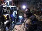
Inside NASA’s Operation IceBridge P3 plane. [Photo Credits: NASA/Icebridge]
-
-
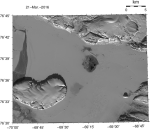
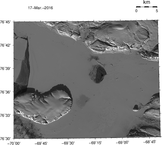
LandSat photo/map of Thule, Greenland Mar.-21, 2016. The airfield of Thule Air Force Base is seen near the bottom on the right. The island in ice-covered Westenholme Fjord is Saunders Island (bottom left) while the glacier top right is Chamberlin Gletscher.
-
-
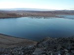
Thule AFB at Pitufik as seen from atop Dundas Mountain Sept.-2, 2015. Note the tidal mud-flats at low tide next to the pier.
-

-
Petermann Gletscher at dawn on 5 Oct. 2015 as captured by NASA Operation IceBridge. Our Ocean Weather Station is in the corner bottom left.
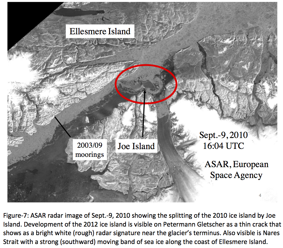
The establishment of military weather stations and airfields in the high Arctic coincided with the discovery of massive ice islands drifting freely in the Arctic Ocean. On Aug.-14, 1946 airmen of the 46th Strategic Reconnaissance Squadron of the US Air Force discovered a moving ice islands with an area of about 200 square that was kept secret until Nov.-1950 (Koenig et al, 1950). Most of these ice islands originated from rapidly disintegrating ice shelves to the north of Ellesmere island (Jeffries, 1992; Copland 2007), however, the first historical description of an ice islands from Petermann Gletscher came from Franz Boas in 1883 who established a German station in Cumberland Sound at 65 N latitude and 65 W longitude as part of the first Polar Year.
![Petermann Ice Island of 2012 at the entrance of Petermann Fjord. The view is to the north-west with Ellesmere Island, Canada in the background. [Photo Credit: Jonathan Poole, CCGS Henry Larsen]](https://icyseas.org/wp-content/uploads/2012/09/pg-iceisland-aug2012_0480.jpg?w=500&h=333)
Petermann Ice Island of 2012 at the entrance of Petermann Fjord. The view is to the north-west with Ellesmere Island, Canada in the background. [Photo Credit: Jonathan Poole, CCGS Henry Larsen]
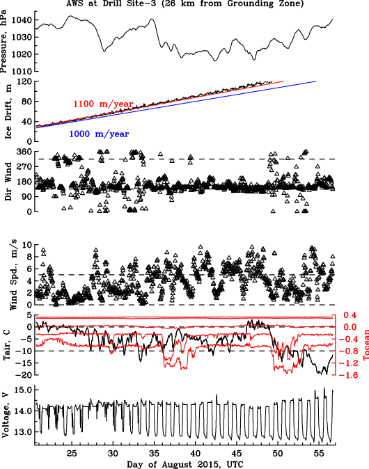
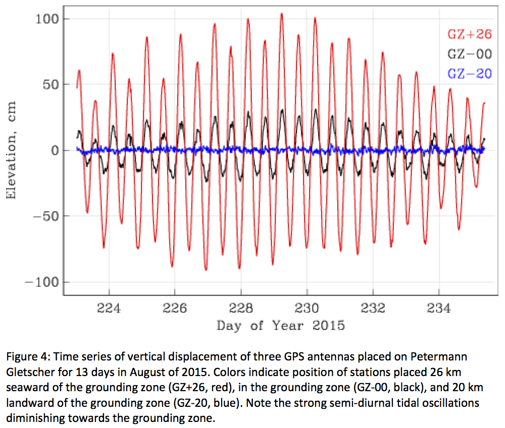
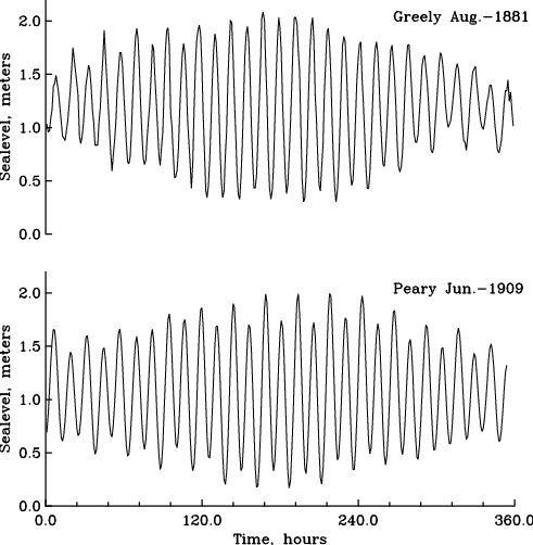
Without knowing the source of the massive tabular iceberg the German physicist Franz Boas reported detailed measurements of ice thickness, extend, and undulating surface features of an ice island in Cumberland Sound that all match scales and characteristics of Petermann Gletscher (Boas, 1885). These characteristics were first described by Dr. Richard Croppinger, surgeon of a British Naval expedition in 1874/75 (Nares, 1876). Dr. Croppinger identified the terminus of Petermann Gletscher as a floating ice shelf when he noticed vertical tidal motions of the glacier from sextant measurements a fixed point (Nares, 1876). His observations on tides were the last until a group of us deployed 3 fancy GPS units on the glacier last summer.
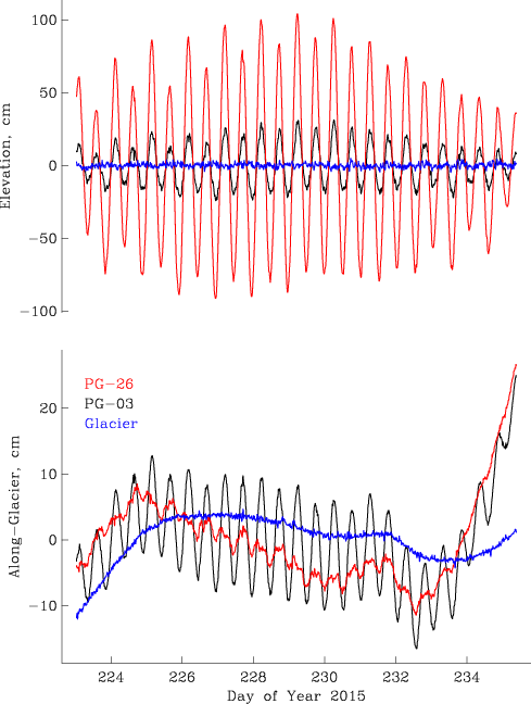
These fancy GPS receivers give centimeter accuracy vertical motions at 30 second intervals. Here is what the deployment of 3 such units in August of 2015 gives me:
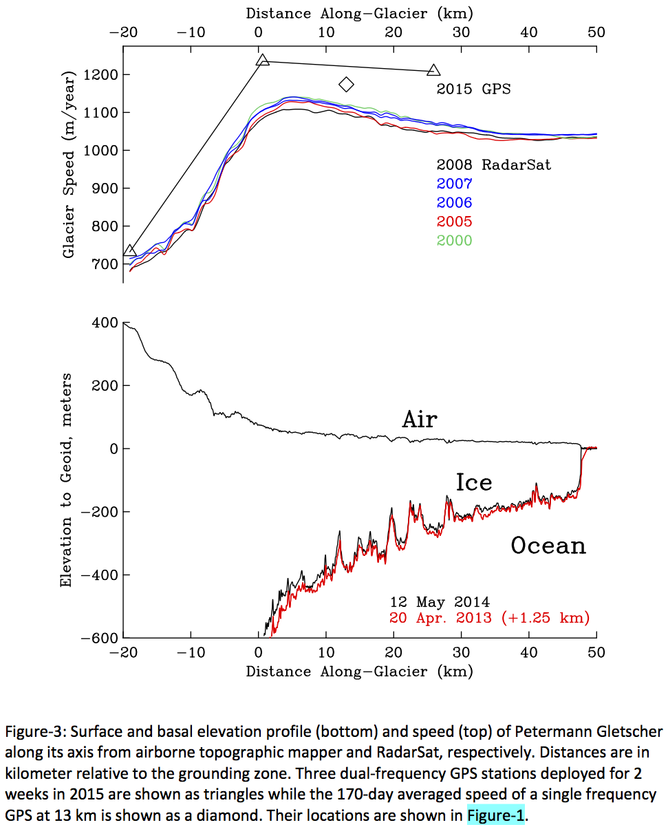
Vertical (top) and horizontal (bottom) motion of Petermann Gletscher from GPS referenced to a GPS base station on bed rock at Kap Schoubye. Note the attenuation of the tide from 26 km sea ward of the grounding line (red) to at the grounding line (black) and 15 km landward of the grounding line (blue). The horizontal location motion has the mean motion removed to emphasize short-term change over the much, much larger forward motion of the glacier that varies from about ~700 (black) to ~1250 meters per year (red).
We have indeed come a far way during the last 150 years or so. Mapping of remote landscape and icescape by starvation and dog-sled has been replaced by daily satellite imagery. Navigation by sextant and a mechanical clock has been replaced by GPS and atomic clock whose errors are further reduced by a local reference GPS. These fancy units and advanced data processing allow me to tell the vertical difference between the top of my iPhone sitting on a table in my garden from the table.

Working at in the garden at home preparing for field work near Petermann Fjord.
P.S.: This is the first in a series of essays that I am currently developing into a peer-reviewed submission to the Oceanography Magazine of the Oceanography Society. The work is funded by NASA and NSF with grants to the University of Delaware.
Ahnert, F. 1963. The terminal disintegration of Steensby Gletscher, North Greenland. Journal of Glaciology 4 (35): 537-545.
Boas, F. 1885. Baffin-Land, geographische Ergebnisse einer in den Jahren 1883 und 1884 ausgeführten Forschungsreise. Petermann’s Mitteilungen Ergänzungsheft 80: 1-100.
Copland, L., D.R. Mueller, and L. Weir. 2007. Rapid loss of the Ayles Ice Shelf, Ellesmere Island, Canada. Geophysical Research Letters 34 (L21501): doi:10.1029/2007GL031809.
Freuchen, P. 1935. Arctic adventures: My life in the frozen North. Farrar & Rinehard, NY, 467 pp.
Higgins, A.K. 1990. North Greenland glacier velocities and calf ice production. Polarforschung 60 (1): 1-23.
Jeffries, M. 1992. Arctic ice shelves and ice islands: Origin, growth, and disintegration, physical characteristics, structural-stratigraphic variability, and dynamics. Reviews of Geophysics 30 (3):245-267.
Johnson, J.P. 1990. The establishment of Alert, N.W.T., Canada. Arctic 43 (1): 21-34.
Koch, L., 1928. Contributions to the glaciology of North Greenland. Meddelelser om Gronland 65: 181-464.
Koenig, L.S., K.R. Greenaway, M. Dunbar, and G. Hattersley-Smith. 1952. Arctic ice islands. Arctic 5: 67-103.
Münchow, A., K.K. Falkner, and H. Melling. 2015. Baffin Island and West Greenland current systems in northern Baffin Bay. Progress in Oceanography 132: 305-317.
Münchow, A., L. Padman, and H.A. Fricker. 2014. Interannual changes of the floating ice shelf of Petermann Gletscher, North Greenland, from 2000 to 2012. Journal of Glaciology 60 (221): doi:10.3189/2014JoG13J135.
Nares, G. 1876. The official report of the recent Arctic expedition. John Murray, London,
Rassmussen, K., 1921: Greenland by the Polar Sea: the Story of the thule Expedition from Melville Bay to Cape Morris Jessup, translated from the Danish by Asta and Rowland Kenney, Frederick A. Stokes, New York, NY, 327 pp.


![Working on the sea ice off northern Greenland [Photo credit, Steffen Olsen]](https://icyseas.org/wp-content/uploads/2016/12/image002.jpg?w=500&h=375)


![An F-102 jet of the 332d Fighter-Interceptor Squadron at Thule AFB in 1960. [Credit: United States Air Force]](https://icyseas.org/wp-content/uploads/2013/06/332d_fighter-interceptor_squadron_-_f-102_-_thule_ab.jpg)
![Petermann Ice Island of 2012 at the entrance of Petermann Fjord. The view is to the north-west with Ellesmere Island, Canada in the background. [Photo Credit: Jonathan Poole, CCGS Henry Larsen]](https://icyseas.org/wp-content/uploads/2012/09/pg-iceisland-aug2012_0480.jpg)

![Dr. Helen Johnson in August 2009 on the pier of Thule AFB with CCGS Henry Larsen and Dundas Mountain in the background. [Credit: Andreas Muenchow]](https://icyseas.org/wp-content/uploads/2013/06/img_0006.jpg)
![Thule AFB with its airport, pier, and ice-covered ocean in the summer. The island is Saunders Island. The ship is most likely the CCGS Henry Larsen in 2007. [Credit: Unknown]](https://icyseas.org/wp-content/uploads/2013/06/thule_air_base_aerial_view.jpg)

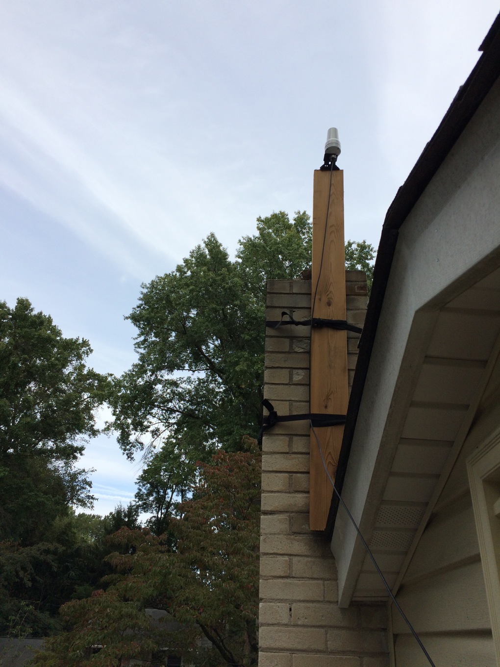
![University of Delaware Ocean-Weather station on Petermann Glacier with the hot-water drilling team UDel and British Antarctic Survey after deployment Aug.-20, 2015 [Credit: Peter Washam, UDel]](https://icyseas.org/wp-content/uploads/2015/09/udel-aows_3052.jpg)