“In 1921 owing to starvation I had to go directly from Cape Heiberg-Juergensen to our cache at Cape Agassiz … during this journey the greater part of the glacier was mapped.” –Lauge Koch, 1928
Petermann Fjord connects Petermann Gletscher to Nares Strait which in turn is connected to the Arctic Ocean in north and the Atlantic Ocean in the south (Figure-2). The track of Petermann ice island PII-2010A emphasizes this connection as the 60 meter thick section of the ice island reaches the Labrador Sea in the south within a year after its calving in 2010.

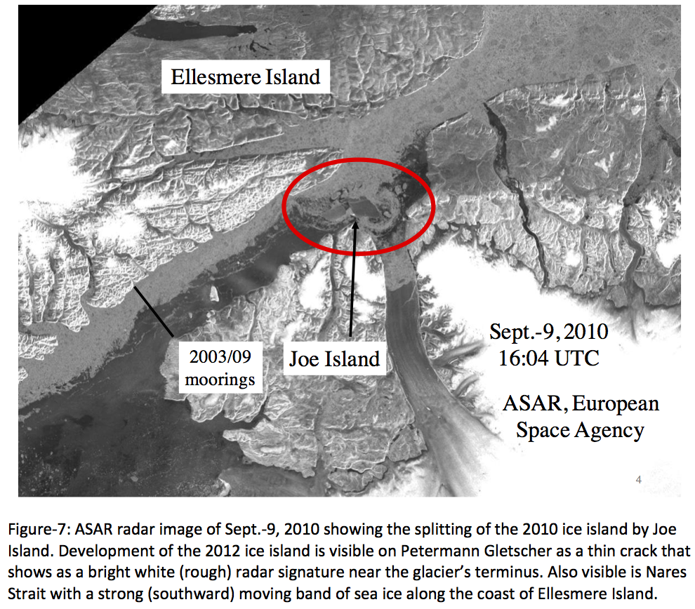
PII-2010 left Petermann Fjord on the 9th of September in 2010 when it broke into segments A and B while pivoting around a real island. It flushed out of Nares Strait 10 days later when an ice-tracking beacon was placed to track the ice island. The ~60 m thick segment PII-2010A moved southward with the Baffin Island Current (Münchow et al., 2015) at an average speed of ~ 0.11 m/s past Davis Strait. Remaining on the continental shelf of the Labrador Sea, it passed Boas’ Cumberland Sound, Labrador, and reached Newfoundland in August 2011 when it melted away in a coastal cove about 3000 km from Petermann Fjord (Figure-2).
Petermann Gletscher drains about 4% of the Greenland ice sheet via a network of channels and streams that extend about 750 km landward from the grounding line (Bamber et al., 2013). The glacier goes afloat at the grounding zone where bedrock, till, and ice meet the ocean waters about 600 meter below sea level (Rignot, 1996).
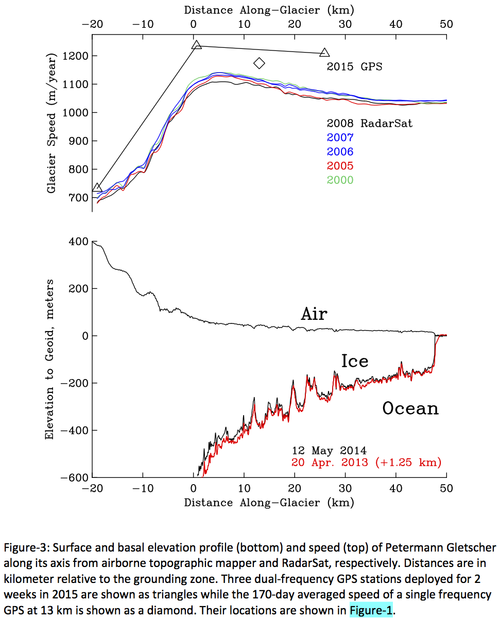
Figure-3 shows a section of surface elevation from a laser altimeter flown on a repeat path along the glacier in April 2013 and May 2014 as part of NASA’s Operation IceBridge. Assuming hydrostatic balance, we also show basal topography below the sea surface that varies from 200 meters at the terminus to 600 meters at the grounding zone near distance zero (Figure-3). The 2013 profile has been shifted seaward by 1.25 km to match the terminus position. Note the close correspondence of large and small crevasses in 2013 and 2014 near 20, 40, and 45 km from the grounding zone.
The seaward shift of the 2013 relative to the 2014 profile implies a uniform glacier speed of about 1180 meters per year. This value is almost identical to the 1170 meters per year that we measure between 20th August of 2015 and 11th February of 2016 with a single-frequency GPS placed about 13 km seaward of the grounding zone as part of the ocean weather observatory.
We compare 2013/14 and 2015/16 velocity estimates in Figure-3 with those obtained from RadarSat interferometry between 2000 and 2008 (Joughin et al., 2010) of which I here only show three:
-

- Speed of Petermann Gletscher for the 2008/09 period from RadarSat interferometry (Joughin et al., 2010). Symbols indicate dual frequency GPS position. Black line near lower center across the glacier indicates the grounding zone.
-

- Speed of Petermann Gletscher for the 2005/06 period from RadarSat interferometry (Joughin et al., 2010). Symbols indicate dual frequency GPS position. Black line near lower center across the glacier indicates the grounding zone.
-

- Speed of Petermann Gletscher for the 2000/01 period from RadarSat interferometry (Joughin et al., 2010). Symbols indicate dual frequency GPS position. Black line near lower center across the glacier indicates the grounding zone.
Figure-3 shows that glacier speeds before 2010 are stable at about 1050 m/y, but increased by about 11% after the 2010 and 2012 calving events. This increase is similar to the size of seasonal variations of glacier motions. Each summer Petermann Gletscher speeds up, because surface meltwater percolates to the bedrock, increases lubrication, and thus reduces vertical friction (Nick et al., 2012). Figure 3 presents summer velocity estimates for August of 2015 from three dual-frequency GPS. The along-glacier velocity profiles measured by these geodetic sensors in the summer follow the shape of the 2000 to 2008 winter record, however, its speeds are about 10% larger and reach 1250 m/y near the grounding zone (Figure 3).
-

- Petermann Gletscher August 10, 2015 with center channel in foreground.
-

- Camping site of the ice drilling team on Petermann Gletscher in August 2015 during installation of the Ocean Weather Station. [Credit: Peter Washam]
-

- UNAVCO GPS systems for deployment on Petermann Gletscher.
-

- Petermann Gletscher at dawn on 5 Oct. 2015 as captured by NASA Operation IceBridge. Our Ocean Weather Station is in the corner bottom left.
-

- Terminus of Petermann Gletscher with Hubert (right), Belgrave (center), and Un-Named (left) Glaciers coming in from Hall Land in the north. The ocean is to the left (west).
-

- View across Petermann Gletscher from west to east near Site-C where we deployed two ocean sensors on Aug.-9, 2015.
Uncertainty in velocity of these GPS systems is about 1 m/y which we estimate from two bed rock reference stations 82 km apart. Our ice shelf observations are referenced to one of these two semi-permanent geodetic stations. Its location at Kap Schoubye is shown in Figure-1. Data were processed using the GAMIT/TRACK software distributed by MIT following methodology outlined by King (2004) to archive vertical accuracy of 2-3 centimeters which, we show next, is small relative to tidal displacements that reach 2 meters in the vertical.
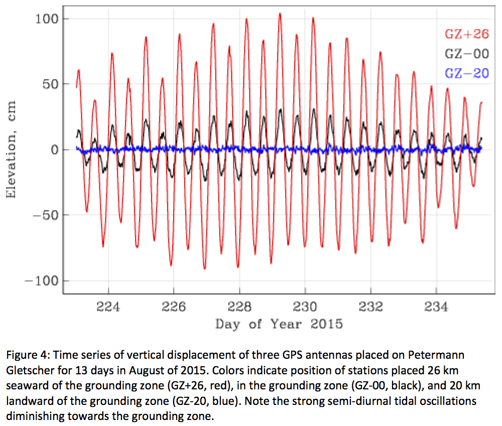
Figure-4 shows the entire 13 day long record of vertical glacier displacement from 30 seconds GPS measurements in August of 2015. The observed range of vertical glacier displacements diminishes from almost 2 meters about 26 km seaward of the grounding zone (GZ+26) via 0.6 meters in the grounding zone (GZ-00) to nil 20 km landward of the grounding zone (GZ-20). Anomalies of horizontal displacement are largest at GZ-00 with a range of 0.2 m (not shown) in phase with vertical oscillations (Figure-4).
More specifically, at GZ+26 we find the ice shelf to move up and down almost 2 meters roughly twice each day. This is the dominant semi-diurnal M2 tide which has a period of 12.42 hours. Notice that for each day there is also a diurnal inequality in this oscillation, that is, the two maximal (minimal) elevations oscillate from a higher to a lower High (Low) water. This is the diurnal K1 tide which has a period of 23.93 hours. And finally, all amplitudes appear modulated by some longer period that appears close to the record length of almost two weeks. This is the spring-neap cycle that is caused by a second semi-diurnal S2 tide that has a period of 12.00 hours. A formal harmonic analysis to estimate the amplitude and phases of sinusoidal oscillations at M2, K1, S2 and many more tidal constituents will be published elsewhere for both Petermann Fjord and Nares Strait. Preliminary results (not shown) reveal that the amplitudes and phases of the tidal signals at GZ+26 are identical to those observed off Ellesmere Island at 81.7 N latitude in both the 19th (Greely, 1888) and 21st century.
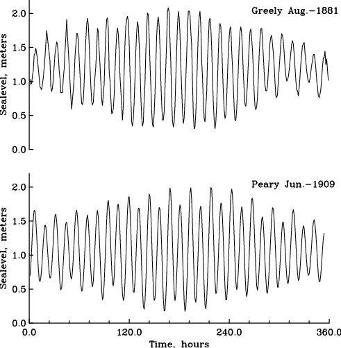
Hourly tidal observations at Discovery Harbor taken for 15 days by Greely in 1881 and Peary in 1909.
In summary, both historical and modern observations reveal real change in the extent of the ice shelf that moves at tidal, seasonal, and interannual time scales in response to both local and remote forcing at these times scales. Future studies will more comprehensively quantify both the time rate of change and its forcing via formal time series analyses.
P.S.: This is the second in a series of four essays that I am currently developing into a peer-reviewed submission to the Oceanography Magazine of the Oceanography Society. The work is funded by NASA and NSF with grants to the University of Delaware.
References:
Bamber, J.L., M.J. Siegert, J.A. Griggs, S. J. Marshall, and G. Spada. 2013. Palefluvial mega-canyon beneath the central Greenland ice sheet. Science 341: 997-999.
Greely, A.W. 1888. Report on the Proceedings of the United States Expedition to Lady Franklin Bay, Grinnell Land. Government Printing Office, Washington, DC.
Joughin, I., B.E. Smith, I.M. Howat, T. Scambos, and T. Moon. 2010. Greenland flow variability from ice-sheet wide velocity mapping. Journal of Glaciology 56 (197): 415-430.
King, B. 2004. Rigorous GPS data-processing strategies for glaciological applications. Journal of Glaciology 50 (171): 601–607.
Münchow, A., K.K. Falkner, and H. Melling. 2015. Baffin Island and West Greenland current systems in northern Baffin Bay. Progress in Oceanography 132: 305-317.
Nick, F.M., A. Luckman, A. Vieli, C.J. Van Der Veen, D. Van As, R.S.W. Van De Wal, F. Pattyn, A.L. Hubbard, and D. Floricioiu. 2012. The response of Petermann Glacier, Greenland, to large calving events, and its future stability in the context of atmospheric and oceanic warming. Journal of Glaciology 58 (208): 229-239.
Rignot, E. 1996. Tidal motion, ice velocity and melt rate of Petermann Gletscher, Greenland, measured from radar interferometry. Journal of Glaciology 42 (142): 476-485.

![Ice fields seen in Labrador Current April 6, 2008 from a plane. [Photo Credit: Daniel Schwen]](https://icyseas.org/wp-content/uploads/2013/05/labrador_current.jpg)
![USCGC Marion built in 1927 [from http://laesser.org/125-wsc/]](https://icyseas.org/wp-content/uploads/2013/03/marion.jpg)
![Iceberg in the fog off Upernarvik, Greenland in July of 2003. [Photo Credit: Andreas Muenchow]](https://icyseas.org/wp-content/uploads/2013/03/helen2003upernarvik.jpg)
![Dr Helen Johnson on acoustic Doppler current profiler (sonar to measure ocean velocity) watch aboard the USCGC Healy in Baffin Bay in 2003. [Photo credit: Andreas Muenchow]](https://icyseas.org/wp-content/uploads/2013/03/helen2003adcp.jpg)


