Death by starvation, drowning, and execution was the fate of 19 members of the US Army’s Lady Franklin Bay Expedition that was charged in 1881 to explore the northern reaches of the American continent. Only six members returned alive, however, they carried papers of tidal observations that they had made at Discovery Harbor at almost 82 N latitude, less than 1000 miles from the North Pole. Air temperatures were a constant -40 (Fahrenheit or Celsius) in January and February. While I knew and wrote of this most deadly of all Arctic expeditions, only 2 days ago did I discover a brief 1887 report in Science that a year-long record of hourly tidal observations exist. How to find these long forgotten data?
-

-
“House at Conger, East side, March 1882” by George W. Rice, from Library of Congress, http://www.loc.gov/item/2006676100/
-

-
Sea-ice foot at Distant Cape near Discovery Harbor in June, 1882. Photo by G.W. Rice, Library of Congress.
-

-
Temperature (black) and pressure (red) record for a year at Discovery Harbor (Fort Conger) on northern Ellesmere Island, Canada. From http://www.arctic.noaa.gov/aro/ipy-1/
My first step was to search for the author of the Science paper entitled “Tidal observations of the Greely Expedition.” Mr. Alex S. Christie was the Chief of the Tidal Division of the US Coast and Geodedic Survey. He received a copy of the data from Lt. Greely. His activity report dated June 30, 1887 confirms receipt and processing of the data, but he laments about “deficient computer power” and requests “two computers of standard ability preferable by young men of 16 to 20 years.” Times and language have changed: In 1887 a computers was a man hired to crunch numbers with pen and paper.

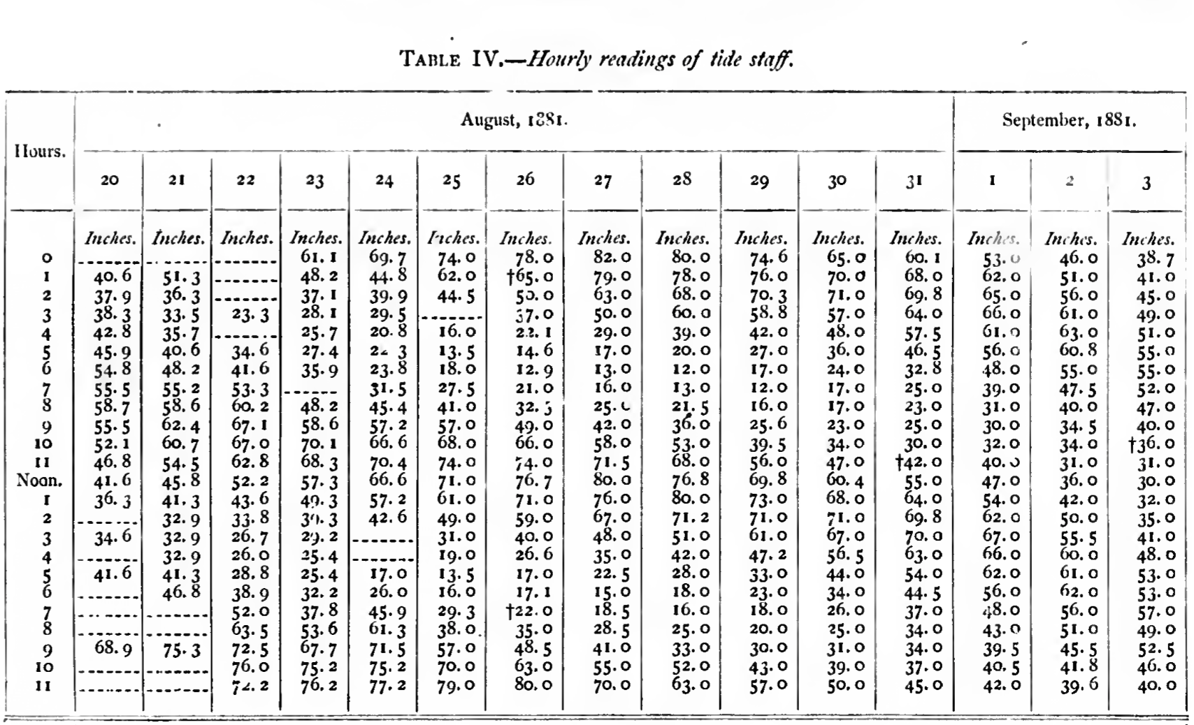
Data table of 15 days of hourly tidal sea level observations extracted from Greely (1888).
While somewhat interesting, I still had to find the real data shown above, but further google searches of the original data got me to the Explorer’s Club in New York City where in 2003 a professional archivist, Clare Flemming, arranged and described the “Collection of the Lady Franklin Bay Expedition 1881-1884.” This most instructive 46 page document lists the entire collection of materials including Series III “Official Research” that consists of 69 folders in 4 Boxes. Box-4 File-15 lists “Manuscript spreadsheet on Tides, paginated. Published in Greely (1888), 2:651-662” as well as 3 unpublished files on tides and tide gauges. With this reference, I did find the official 1888 “Report on the United States Expedition to Lady Franklin Bay” of the Government Printing Office as digitized from microfiche as
https://archive.org/details/cihm_29328
which on page 641 shows the above table. There are 19 more tables like it, but at the moment I have digitized only the first one. Unlike my colleagues at the US Coast and Geodedic Survey in 1887, I do have enough computer power to graph and process these 15 days of data in mere seconds, e.g.,

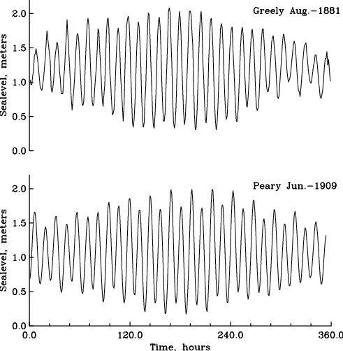
Hourly tidal observations at Discovery Harbor taken for 15 days by Greely in 1881 and Peary in 1909.
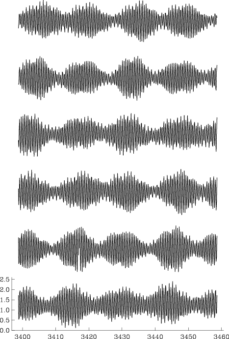
A more technical “harmonic” analyses reveals that Greely’s 1881 (or Peary’s 1909) measured tides at Discovery Harbor have amplitudes of about 0.52 m (0.59) for the dominant semi-diurnal and 0.07 m (0.12) for the dominant diurnal oscillation. My own estimates from a 9 year 2003 to 2012 record gives 0.59 and 0.07 m for semi-diurnal and diurnal components. This gives me confidence, that both the 1881 and 1909 data are good, just have a quick look at 1 of the 9 years of data I collected:

Tidal sea level data from a pressure sensor placed in Discovery Harbor in 2003. Each row is 2 month of data starting at the top (August 2003) and ending at the bottom (July 2004).
There is more to this story. For example, what happened to the complete and original data recordings? Recall that Greely left Discovery Harbor late in the fall of 1883 after supply ships failed to reach his northerly location two years in a row. This fateful southward retreat from a well supplied base at Fort Conger and Discovery Harbor killed 19 men. Unlike ghostly Cape Sabine where most of the men perished, Discovery Harbor had both local coal reserves and musk ox in the nearby hills that could have provided heat, energy, and food for many years.
It amazes me, that a 1-year copy of tidal data survived the death march of Greely’s party. It took another 18 years for the complete and original records to be recovered by Robert Peary who handed them to the Peary Arctic Club which in 1905 morphed into Explorer’s Club of New York City. I suspect (but do not know), that these archives contain another 2 years of data that nobody but Edward Israel in 1882/83 and the archivist in 2003 laid eyes on. Sergeant Edward Israel was the astronomer who collected the original tidal data. He perished at Cape Sabine on May 29, 1884, 25 years of age.

Edmund Israel, astronomer of the Lady Franklin Bay Expedition of 1881-1884.
References:
Christie, A.S., 1887: Tidal Observations of the Greely Expedition, Science, 9 (214), 246-249.
Greely, A.W., 1888: Report on the Proceedings of the United States Expedition to Lady Franklin Bay, Grinnell Land, Government Printing Office, Washington, DC.
Guttridge, L., 2000: The ghosts of Cape Sabine, Penguin-Putnam, New York, NY, 354pp.
![Dr. Helen Johnson in August 2009 on the pier of Thule AFB with CCGS Henry Larsen and Dundas Mountain in the background. [Credit: Andreas Muenchow]](https://icyseas.org/wp-content/uploads/2013/06/img_0006.jpg)
![Thule AFB with its airport, pier, and ice-covered ocean in the summer. The island is Saunders Island. The ship is most likely the CCGS Henry Larsen in 2007. [Credit: Unknown]](https://icyseas.org/wp-content/uploads/2013/06/thule_air_base_aerial_view.jpg)