Author Archives: Andreas Muenchow

Petermann Gletscher Ocean Station Revisited

Standing on floating Petermann Gletscher last sunday, I called my PhD student Peter Washam out of bed at 5 am via our emergency Iridium phone to check the machine that Keith Nicholls and I had just repaired. We had prepared for this 4 months and quickly established that a computer in Delaware could “talk” to a computer in Greenland to receive data from the ocean 800 m below my feet on a slippery glacier. For comparison the Empire State Building is 480 m high. The closest bar was 5 hours away by helicopter at Thule Air Force Base from where Keith and I had come.
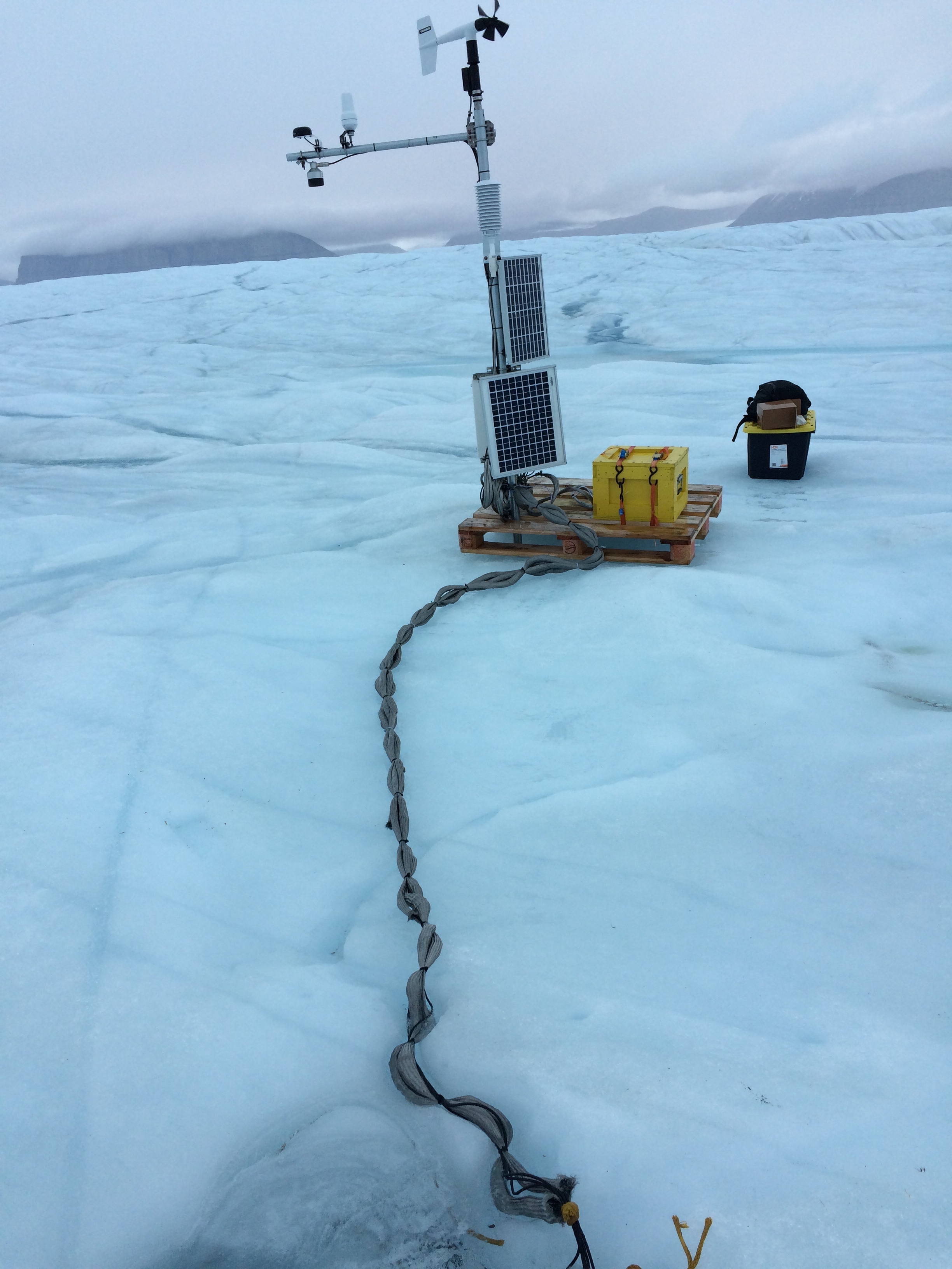
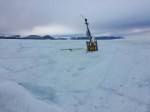
Cabled ocean observatory linked to a University of Delaware weather station on Petermann Gletscher, Greenland on 28 August 2016. View is to the north.

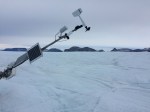
Refurbished ocean observatory linked via cables to a University of Delaware weather station on Petermann Gletscher, Greenland on 28 August 2016. View is to the north.

Remote Petermann Gletscher can be reached by helicopter only of one prepares at least two refueling stations along the way. Anticipating a potential future need, we had placed 1300 and 1600 liters of A1 jet fuel at two points from aboard the Swedish icebreaker Oden in 2015. The fuel was given to Greenland Air with an informal agreement that we could use the fuel for a 2016 or 2017 helicopter charter. Our first pit stop looked like this on the southern shores of Kane Basin
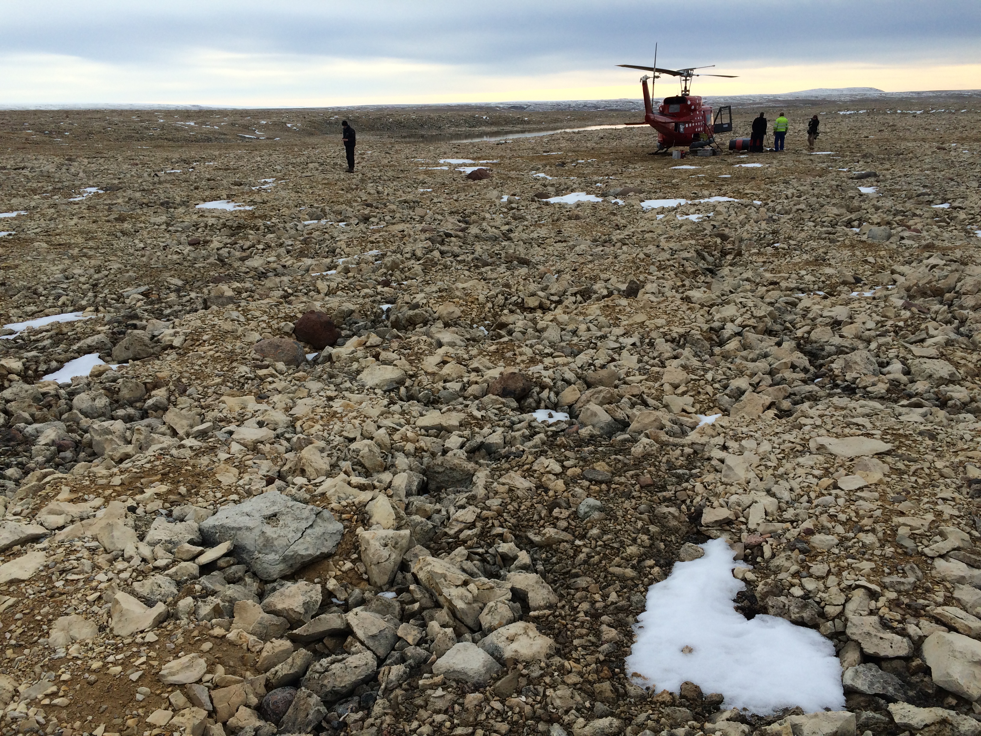
Refueling stop on north-eastern Inglefield Land on 27 August 2016. Air Greenland Bell-212 helicopter in the background, view is to the north.

Refueling stop on southern Washington Land on 27 August 2016. Air Greenland Bell-212 helicopter in the background, view is to the south towards Kane Basin.
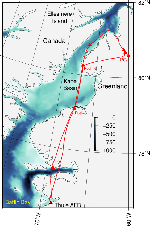
Helicopter flight path on 27/28 August 2016 to reach Petermann Gletscher (PG) via southern (Fuel-S) and northern (Fuel-N) fuel stops in northern Inglefield and southern Washington Land, respectively. Background color is ocean bottom depth in meters.

Helicopter flight path on 27/28 August 2016 to reach Petermann Gletscher (PG) via southern (Fuel-S) and northern (Fuel-N) fuel stops in northern Inglefield and southern Washington Land, respectively. Background color is ocean bottom depth in meters.

Upon arrival at the first (northern-most) Peterman Gletscher (PG) station we quickly confirmed our earlier suspicion that vertical motion within the 100 m thick glacier ice had ruptured the cables connecting two ocean sensors below the ice to data loggers above. We quickly disassembled the station and moved on to our central station that failed to communicate with us since 11 February 2016. Keith predicted that here, too, internal glacier motions would have stretched the cables inside the ice to their breaking point, however, this was not to be the case.

My first impression of this station was one of driftwood strewn on the beach of an ocean of ice:

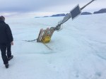
Looks can be deceiving, however, and we found no damage to any electrical components from the yellow-painted wooden battery box housing two 12 Volt fancy “car batteries” at the bottom to the wind sensor on the top. Backed-up data on a memory card from one of two data loggers (stripped down computers that control power distribution and data collections) indicated that everything was working. The ocean recording from more than 800 meters below our feet was taken only a few minutes prior. In disbelief Keith and I were looking over a full year-long record of ocean temperature, salinity, and pressure as well as glacier motions from a GPS. This made our choices on what to do next very simple: Repair the straggly looking ocean-glacier-weather station, support it with a metal pole drilled 3.5 m into the glacier ice, and refurbish the adjacent radar station. We went to work for a long day and longer night without sleep.
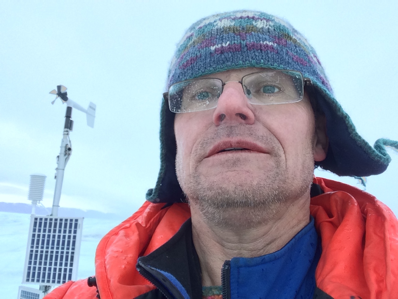
Selfie on Petermann Gletscher on sunday 28 August 2016 after 33 hours without sleep. Weather station and northern wall of Petermann in the clouds. It was raining, too.

Selfie on Petermann Gletscher on sunday 28 August 2016 after 33 hours without sleep. Weather station and northern wall of Petermann in the clouds. It was raining, too.

When all was done, University of Delaware graduate student Peter Washam did the last check at 5:30 am sunday morning. Since then our Greenland station accepts Iridium phone calls every three hours, sends its data home where I post it daily at

http://ows.udel.edu

The data from this station will become the center piece of Peter’s dissertation on glacier-ocean interactions. Peter was part of the British hot water drilling team who camped on the ice in 2015 for 3 weeks while I was on I/B Oden responsible for the work on the physical oceanography of the fjord and adjacent Nares Strait. Alan Mix of Oregon State University prepared and led the 2015 expedition giving us ship and helicopter time generously to support our work on the ice shelf of Petermann. Saskia Madlener documented the scope of the 2015 work in a wonderful set of three videos

Ocean & Ice – https://vimeo.com/178289799
Rocks & Shells – https://vimeo.com/178379027
Seafloor & Sediment – https://vimeo.com/169110567

A first peer-reviewed publication on this station and its data until 11 February 2016 will appear in the December 2016 issue of the open-access journal Oceanography with the title The Ice Shelf of Petermann Gletscher, North Greenland and its Connection to the Arctic and Atlantic Oceans.
Oceanography and Price of Milk at Thule Air Force Base, Greenland

Looking ahead across Greenland’s ice sheet and glaciers and sea ice, I fell in love with Thule Air Force Base when I was stranded there last year. The people I met on base during these 2 days both military and civilian, both American and Danish, were incredible in how they shared their time, their houses, their huts, their containers, their beaches, their hills, and most of all their pride in working together on something special in a hostile, isolated, and beautiful place that is Thule and adjacent Dundas, Greenland. It is stunning to me, however, that this prime location next to a large airfield, next to a deep water port, next to tidewater glaciers, and next to the open, albeit ice-covered ocean has not been used much for field work in oceanography on ice-ocean-glacier interactions. This needs change.

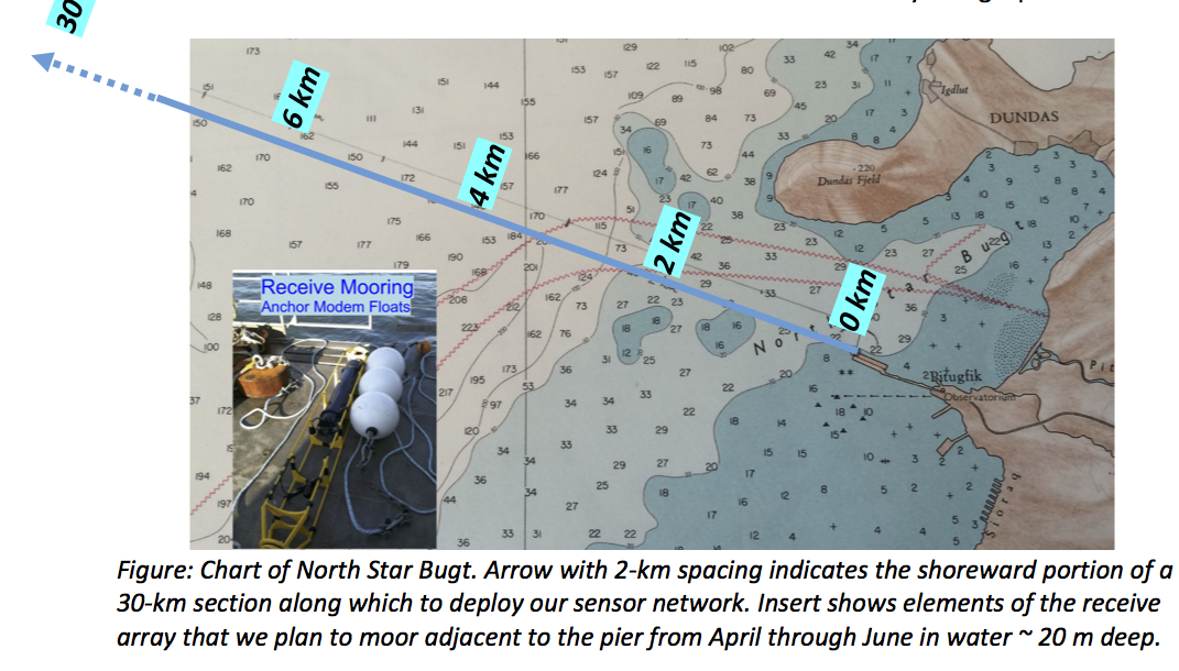
The two days last year in Thule allowed me to walk around and explore for the first and only time in the 12 years that I passed through Thule to board or leave icebreakers working far to the north in Nares Strait and at Petermann Gletscher. Thule is the northern-most deep water port in the world and I have written about some of its Cold War histories, its long, wood-decked pier, and its hikes. My interest in Thule and its pier emerged when the National Science Foundation funded an experimental engineering program on how to send e-mails underwater from one ocean sensor to another much like the way we all do it through the air with our smart cell phones. We want to test this system under the ice and there is plenty of ice around Thule for most of the year.

Thule-NSF2017

LandSat photo/map of Thule, Greenland Mar.-21, 2016. The airfield of Thule Air Force Base is seen near the bottom on the right. The island in ice-covered Westenholme Fjord is Saunders Island (bottom left) while the glacier top right is Chamberlin Gletscher.

LandSat photo/map of Thule, Greenland Mar.-21, 2016. The airfield of Thule Air Force Base is seen near the bottom on the right. The island in ice-covered Westenholme Fjord is Saunders Island (bottom left) while the glacier top right is Chamberlin Gletscher.

While all this sounds like fun, how does one get stuff like oneself or sensors, or rope, or an entire container of gear to Thule. This turns out to be very tricky as there are no roads to get there, the port is ice-free only from June through October, and the ~600 people living here and another 600 living 60 miles over a mountain and several glaciers to the north do not exactly support a competitive market of air carriers. There is a reason that a gallon of milk should cost $80 were it not subsidized by the US Department of Defence. Actual shipping costs of such items are $10 per pound (452 grams) by air and a gallon of milk weights about 8 pounds. So, if I have 1000 pounds of gear, say, I’d have to pay $10,000 just get it to Thule. For context, I am about to ship 15,000 pounds of oceanographic gear to Seattle for an experiment in the Arctic Ocean later this fall. So, air shipment is not really practical for larger experiments, however, this is

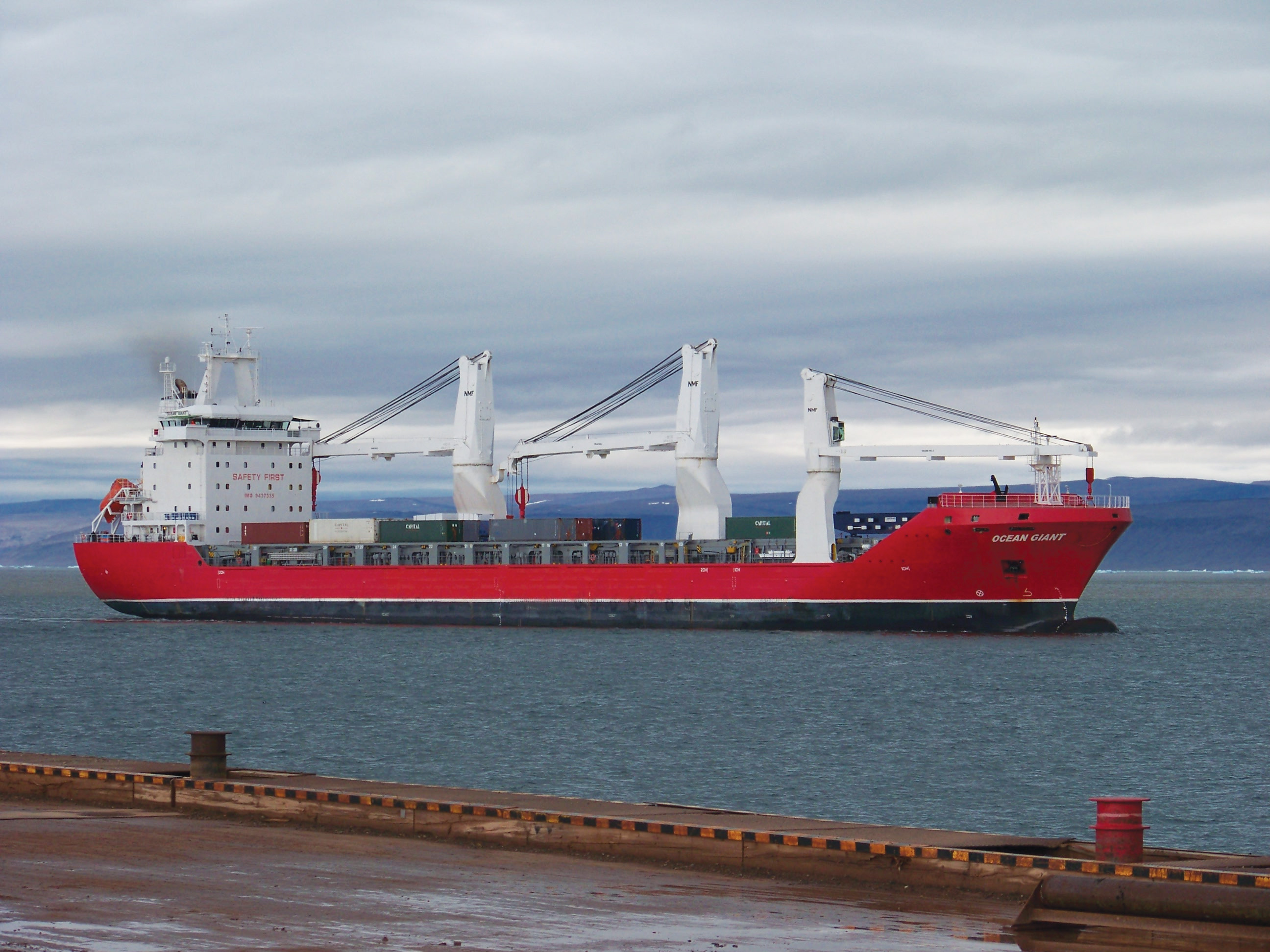
which is Operation “Pacer Goose” run by the US Navy SeaLift Command. Once every year in early July it provides the bulk of supplies and fuel to remote Thule Air Force Base. Think container-sized stuff. It is also the reason, that my experiment in the coastal waters of Wolstenholme Fjord should not be in the way of this annual event that uses the pier. Here is the M/V Ocean Giant as seen from the pier at Thule:

100_0287

My only problem now is that to use this container ship, the earliest possible date to use the container I may want to ship is in the fall of 2017. So, do I want to do oceanography while walking and driving on water frozen solid by sea ice in March and April … or is there a way to deploy my oceanographic sensors via a small boat in the open waters in the fall? New ideas and questions to ponder. This, however, is always fun, too many ideas, each new problem is also an opportunity to do things differently, perhaps. And a good, solid, and comprehensive oceanographic study of the waters off Thule is, I feel, overdue. [I also need to talk to my Danish friends and colleagues about this, more ideas yet.]

Sea ice and 2016 Arctic field work

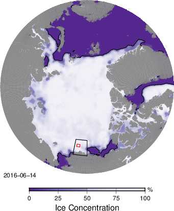
The sea ice in the Arctic Ocean is quickly disappearing from coastal areas as we are entering the summer melt season. This year I follow this seasonal event with nervous anticipation, because in October and November we will be out at sea working north of northern Alaska. We plan to deploy a large number of ocean sensors to investigate how sound propagates from the deep Arctic Ocean on to the shallow Chukchi Sea. This figure shows our study area with the ice cover as it was reported yesterday from space:

Ice concentration for June 14, 2016 from SSM/I imagery. Insert show study area to the north of Alaska and planned mooring locations (red box).

Ice concentration for June 14, 2016 from SSM/I imagery. Insert show study area to the north of Alaska and planned mooring locations (red box).

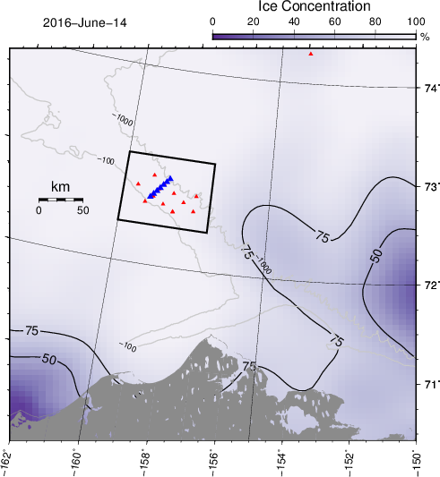
Zooming in a little further, I show the coast of Alaska along with 100 and 1000 meter contour of bottom depth over a color map of ice concentrations:

Ice concentrations from SSM/I to the north of norther Alaska with planned mooring locations across the sloping bottom. The 100 and 1000 meter contours are shown in gray with blue and red symbols representing locations of ocean and acoustic sensors, respectively.

Ice concentrations from SSM/I to the north of norther Alaska with planned mooring locations across the sloping bottom. The 100 and 1000 meter contours are shown in gray with blue and red symbols representing locations of ocean and acoustic sensors, respectively.

My responsibilities in this US Navy-funded project are the seven densely packed blue triangles. They indicate locations where I hope to measure continuously for a year ocean temperature, salinity, and pressure from which to construct sections of speed of sound and how it varies in time and space. I will also measure ice draft as well ice and ocean currents from which to estimate the roughness of the sea ice over time. Sea ice and ocean properties both impact sound propagation from deep to shallow water and vice versa.

A first question: What will the ice be like when we get there? This is the question that has the 40 or so people all working on this project anxiously preparing for the worst, but how can we expect what challenges are to come our way?

Doing my homework, I downloaded from the National Snow and Ice Data Center all gridded maps of ice concentrations that microwave satellites measured almost daily since 1978. Then I crunch the numbers on my laptop with a set of kitchen-sink Unix tools and code snippets such as

set ftp = 'ftp://sidads.colorado.edu'
set dir = 'pub/DATASETS/nsidc0081_nrt_nasateam_seaice/north'
...
wget -r -nd -l1 --no-check-certificate $ftp/$dir/$year/$file

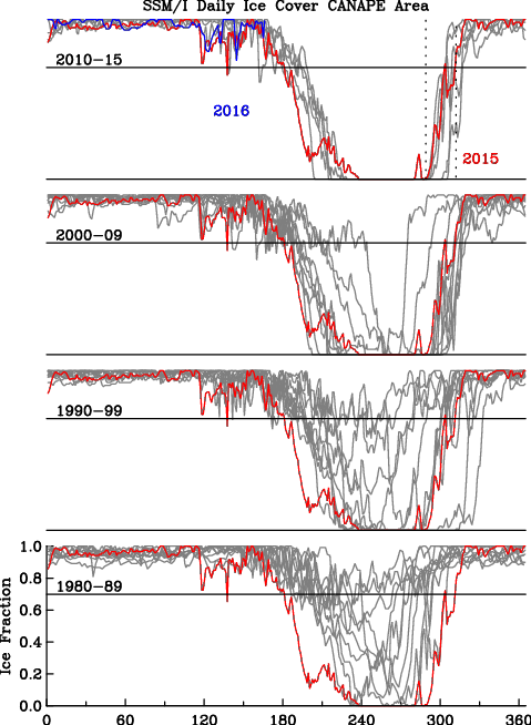
along with fancy and free Fortran and General Mapping Tools to make the maps shown above. With these tools and data I can then calculate how much sea ice covers any area at any time. The result for custom-made mooring area at almost daily resolution gives a quick visual that I use to prepare for our fall 2016 expedition. The dotted lines in the top panel indicate the dates we are in the area.

Time series of daily ice concentration in the study area for different decades from January-1 through Dec.-31 for each year from 1980 through 2015. Panels are sorted by decade. The red curve is for 2015 and is shown for comparison in all panels.

Time series of daily ice concentration in the study area for different decades from January-1 through Dec.-31 for each year from 1980 through 2015. Panels are sorted by decade. The red curve is for 2015 and is shown for comparison in all panels.

The story here is well-known to anyone interested in Arctic sea ice and climate change, but here it applies to a tiny spec of ocean between the 100 and 1000 meter isobath where we plan to deployed ocean sensors for a year in the fall of 2016. For the two decades of the last century, the ice cover looks like a crap shoot with 80% ice cover possible any month of the year and ice-free conditions unlikely but possible here or there for a week or two at most. The situation changed dramatically since about 2000. During the last six years our study area has always been free of ice from late August to early October, however, our 2016 expedition is during the transition from ice-free October to generally ice-covered early November, but, I feel, our saving grace is that the sea ice will be thin and mobile. I thus feel that we probably can work comfortable on account of ice for the entire period, but the winds and waves will blow us away …

Weather will be most uncomfortable, because fall is the Pacific storm season. And with little or only thin ice, there will be lots and lots of waves with the ship pitching and rolling and seeking shelter that will challenge us from getting all the work done even with 7 days for bad weather built into our schedule.

I worked in this area on larger ships in 1993, 2003, and in 2004. Here is a photo that Chris Linder of Woods Hole Oceanographic Institution took during a massive storm in the general vicinity in October of 2004. The storm halted all outside work on the 420 feet long USCGC Healy heading into the waves for 42 long and miserable hours:

Icebreaker taking on waves on the stern during a fall storm in the Beaufort Sea in October 2004. [Photo Credit: Chris Linder, Woods Hole Oceanographic Institution]

Icebreaker taking on waves on the bow during a fall storm in the Beaufort Sea in October 2004. [Photo Credit: Chris Linder, Woods Hole Oceanographic Institution]

Oh, I now also recall that during this four-week expedition we never saw land or the sun. It was always a drizzly gray ocean on a gray horizon. The Arctic Ocean in the fall is an often cruel and inhospitable place with driving freezing rain and fog.

How to Power Modern Economies: Read Your Meter

Read you meter at home. This fun-filled advice was given by Sir David MacKay in a wonderful TEDx talk about how we heat our homes, get to work, run our computers, and how it all scales across countries and continents. The idea is really about how we run our lives while also trying to pass on a livable planet to our grand-children without the politically correct “greenwash” and self-righteous “claptraps”. Read your meter, do some algebra, and embrace the adventure to explore your home, your life, and the energy it all takes. If you read this far, watch the movie

David MacKay taught physics and information theory at the University of Cambridge in England. I learnt of him via Ruth Mottram in one of her many tweets. Dr. Mottram studies climate impacts of Greenland glaciers and works at the Danish Meteorological Institute. The tweet made me buy the book “Information Theory, Inference, and Learning Algorithm’s” that David MacKay wrote a few years back. It arrived today.

What piqued my interest was the advanced math that goes into designing networks that send and transform information such telephone calls via wireless, computer networks, and how to deal with imperfect channels of communication. My marriage comes to mind, too, because what I say is not always what I mean which is not always what my wife hears and vice versa, but I digress. Imperfect communication channels are one challenge we will face in an experiment to explore acoustic underwater data transmissions that hopefully will take place next year out of Thule Air Force Base, Greenland. Water and ice are imperfect communication channels that we need to use wisely to make our whispers carry far. Try to talk to a person across a busy street in Manhattan with all its hustle and bustle; you need to find something smarter and more effective than just simple shouting.

David MacKay wrote a second book that is close to his TEDx talk and is called “Sustainable Energy without the Hot Air.” Experimenting at home like any good physicist does, he discovers that “… the more often I read my meter, the less gas I use!”

There is so much more to this man, his work, and ideas as a physicist with a keen interest in the big picture without skipping the details. Sadly, he died yesterday of cancer too early only 48 years of age.

The Ice Shelf of Petermann Gletscher and its Ocean Below: Descriptions

“In 1921 owing to starvation I had to go directly from Cape Heiberg-Juergensen to our cache at Cape Agassiz … during this journey the greater part of the glacier was mapped.” –Lauge Koch, 1928

Petermann Fjord connects Petermann Gletscher to Nares Strait which in turn is connected to the Arctic Ocean in north and the Atlantic Ocean in the south (Figure-2). The track of Petermann ice island PII-2010A emphasizes this connection as the 60 meter thick section of the ice island reaches the Labrador Sea in the south within a year after its calving in 2010.

TOS2016-Fig2

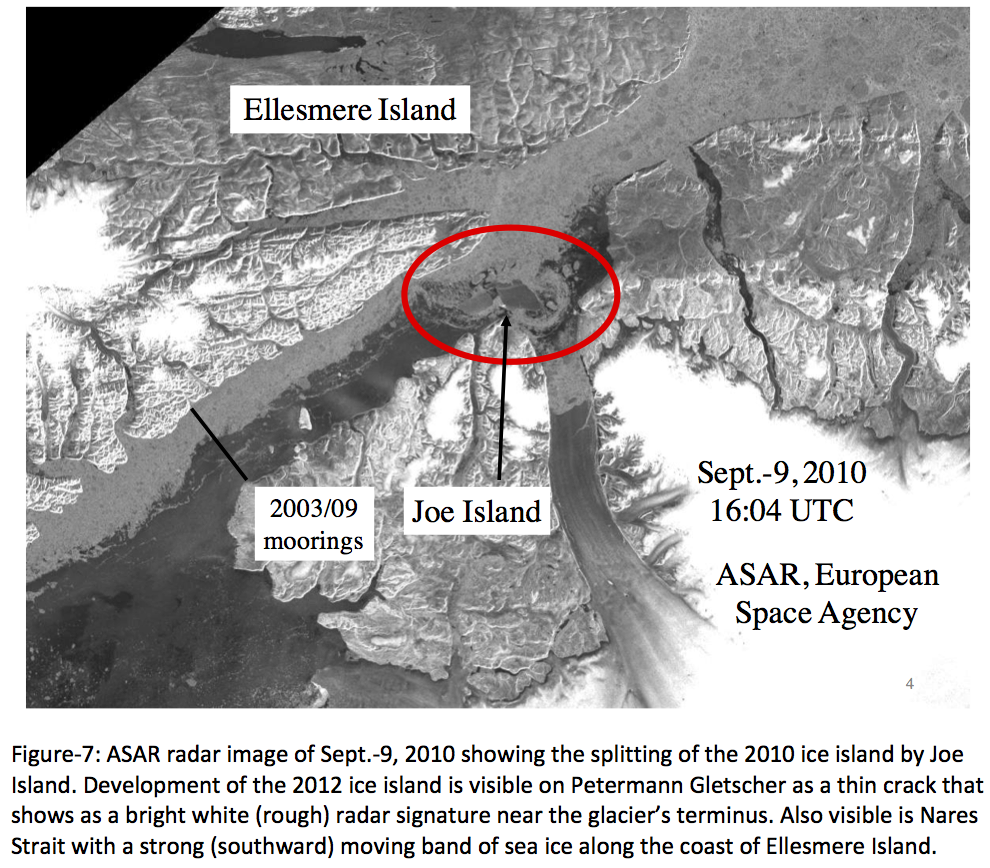
PII-2010 left Petermann Fjord on the 9th of September in 2010 when it broke into segments A and B while pivoting around a real island. It flushed out of Nares Strait 10 days later when an ice-tracking beacon was placed to track the ice island. The ~60 m thick segment PII-2010A moved southward with the Baffin Island Current (Münchow et al., 2015) at an average speed of ~ 0.11 m/s past Davis Strait. Remaining on the continental shelf of the Labrador Sea, it passed Boas’ Cumberland Sound, Labrador, and reached Newfoundland in August 2011 when it melted away in a coastal cove about 3000 km from Petermann Fjord (Figure-2).

TOS2016-Fig7

Petermann Gletscher drains about 4% of the Greenland ice sheet via a network of channels and streams that extend about 750 km landward from the grounding line (Bamber et al., 2013). The glacier goes afloat at the grounding zone where bedrock, till, and ice meet the ocean waters about 600 meter below sea level (Rignot, 1996).

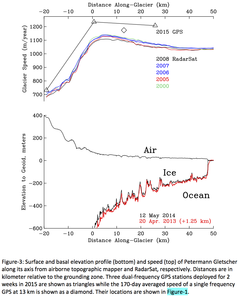
TOS2016-Fig3

Figure-3 shows a section of surface elevation from a laser altimeter flown on a repeat path along the glacier in April 2013 and May 2014 as part of NASA’s Operation IceBridge. Assuming hydrostatic balance, we also show basal topography below the sea surface that varies from 200 meters at the terminus to 600 meters at the grounding zone near distance zero (Figure-3). The 2013 profile has been shifted seaward by 1.25 km to match the terminus position. Note the close correspondence of large and small crevasses in 2013 and 2014 near 20, 40, and 45 km from the grounding zone.

The seaward shift of the 2013 relative to the 2014 profile implies a uniform glacier speed of about 1180 meters per year. This value is almost identical to the 1170 meters per year that we measure between 20th August of 2015 and 11th February of 2016 with a single-frequency GPS placed about 13 km seaward of the grounding zone as part of the ocean weather observatory.

We compare 2013/14 and 2015/16 velocity estimates in Figure-3 with those obtained from RadarSat interferometry between 2000 and 2008 (Joughin et al., 2010) of which I here only show three:

Figure-3 shows that glacier speeds before 2010 are stable at about 1050 m/y, but increased by about 11% after the 2010 and 2012 calving events. This increase is similar to the size of seasonal variations of glacier motions. Each summer Petermann Gletscher speeds up, because surface meltwater percolates to the bedrock, increases lubrication, and thus reduces vertical friction (Nick et al., 2012). Figure 3 presents summer velocity estimates for August of 2015 from three dual-frequency GPS. The along-glacier velocity profiles measured by these geodetic sensors in the summer follow the shape of the 2000 to 2008 winter record, however, its speeds are about 10% larger and reach 1250 m/y near the grounding zone (Figure 3).

Uncertainty in velocity of these GPS systems is about 1 m/y which we estimate from two bed rock reference stations 82 km apart. Our ice shelf observations are referenced to one of these two semi-permanent geodetic stations. Its location at Kap Schoubye is shown in Figure-1. Data were processed using the GAMIT/TRACK software distributed by MIT following methodology outlined by King (2004) to archive vertical accuracy of 2-3 centimeters which, we show next, is small relative to tidal displacements that reach 2 meters in the vertical.

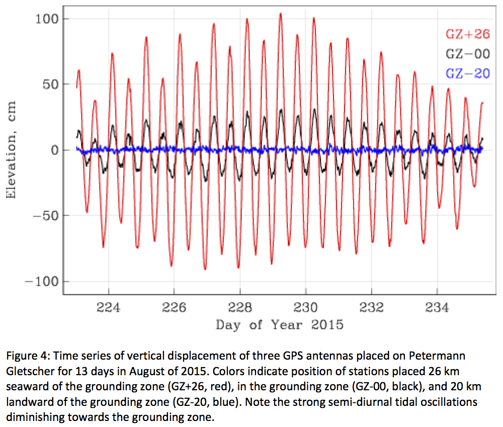
TOS2016-Fig4

Figure-4 shows the entire 13 day long record of vertical glacier displacement from 30 seconds GPS measurements in August of 2015. The observed range of vertical glacier displacements diminishes from almost 2 meters about 26 km seaward of the grounding zone (GZ+26) via 0.6 meters in the grounding zone (GZ-00) to nil 20 km landward of the grounding zone (GZ-20). Anomalies of horizontal displacement are largest at GZ-00 with a range of 0.2 m (not shown) in phase with vertical oscillations (Figure-4).

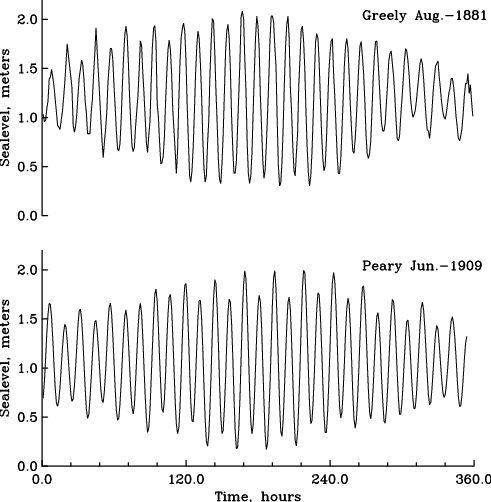
More specifically, at GZ+26 we find the ice shelf to move up and down almost 2 meters roughly twice each day. This is the dominant semi-diurnal M2 tide which has a period of 12.42 hours. Notice that for each day there is also a diurnal inequality in this oscillation, that is, the two maximal (minimal) elevations oscillate from a higher to a lower High (Low) water. This is the diurnal K1 tide which has a period of 23.93 hours. And finally, all amplitudes appear modulated by some longer period that appears close to the record length of almost two weeks. This is the spring-neap cycle that is caused by a second semi-diurnal S2 tide that has a period of 12.00 hours. A formal harmonic analysis to estimate the amplitude and phases of sinusoidal oscillations at M2, K1, S2 and many more tidal constituents will be published elsewhere for both Petermann Fjord and Nares Strait. Preliminary results (not shown) reveal that the amplitudes and phases of the tidal signals at GZ+26 are identical to those observed off Ellesmere Island at 81.7 N latitude in both the 19th (Greely, 1888) and 21st century.

Hourly tidal observations at Discovery Harbor taken for 15 days by Greely in 1881 and Peary in 1909.

Hourly tidal observations at Discovery Harbor taken for 15 days by Greely in 1881 and Peary in 1909.

In summary, both historical and modern observations reveal real change in the extent of the ice shelf that moves at tidal, seasonal, and interannual time scales in response to both local and remote forcing at these times scales. Future studies will more comprehensively quantify both the time rate of change and its forcing via formal time series analyses.

P.S.: This is the second in a series of four essays that I am currently developing into a peer-reviewed submission to the Oceanography Magazine of the Oceanography Society. The work is funded by NASA and NSF with grants to the University of Delaware.

References:

Bamber, J.L., M.J. Siegert, J.A. Griggs, S. J. Marshall, and G. Spada. 2013. Palefluvial mega-canyon beneath the central Greenland ice sheet. Science 341: 997-999.

Greely, A.W. 1888. Report on the Proceedings of the United States Expedition to Lady Franklin Bay, Grinnell Land. Government Printing Office, Washington, DC.

Joughin, I., B.E. Smith, I.M. Howat, T. Scambos, and T. Moon. 2010. Greenland flow variability from ice-sheet wide velocity mapping. Journal of Glaciology 56 (197): 415-430.

King, B. 2004. Rigorous GPS data-processing strategies for glaciological applications. Journal of Glaciology 50 (171): 601–607.

Münchow, A., K.K. Falkner, and H. Melling. 2015. Baffin Island and West Greenland current systems in northern Baffin Bay. Progress in Oceanography 132: 305-317.

Nick, F.M., A. Luckman, A. Vieli, C.J. Van Der Veen, D. Van As, R.S.W. Van De Wal, F. Pattyn, A.L. Hubbard, and D. Floricioiu. 2012. The response of Petermann Glacier, Greenland, to large calving events, and its future stability in the context of atmospheric and oceanic warming. Journal of Glaciology 58 (208): 229-239.

Rignot, E. 1996. Tidal motion, ice velocity and melt rate of Petermann Gletscher, Greenland, measured from radar interferometry. Journal of Glaciology 42 (142): 476-485.