Monthly Archives: January 2012

Heat Sensing Eyes “See” Arctic Ice Thickness

The Arctic sea ice is disappearing before our eyes as we extended them into space in the form of satellites. Every summer for the last few years the area covered by ice is shrinking during the summer when 24 hours of sunlight give us plenty of crisp images. But what about winter? What about now? And does a picture from space tell us how thick the ice is?

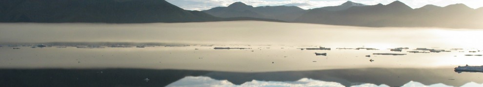
Nares Strait between northern Greenland and Canada on Aug.-13, 2005 with Petermann and Humboldt Glaciers at top and center right from MODIS imagery using red, blue, and green channels.

It is dark in the winter near the north pole as the sun is below the horizon 24 hours each day, but there are many ways to “see” in the dark as flying bats aptly show. They send out sound that bounce off objects from which bats reconstruct objects around them. We use radar from space to do to the same with radio waves to “see” different types of ice at night from satellites. We can also use tiny amounts of heat stored in water, ice, snow, and land to “see” at night. Someone breathing down your neck at a cold dark corner will make our heart beat faster as we “see” the heat not with our eyes, but with our skin. I digress, as I really want to talk about icy Arctic seas and how we can perhaps “see” how thick it is with our eyes in the sky.

The most accurate and pain-staking way to measure ice thickness is drill holes through it. This is back-breaking, manual labor away from the comforts of a ship or a camp. One person watches with a shot-gun for polar bear searching for food, not our food, we are the food. The scientist who does this sweaty, dangerous work on our Nares Strait expeditions is Dr. Michelle Johnston of Canada’s National Research Council. She is a petite, attractive, and smart woman who is calm, competent, and comfortable when she leads men like her bear-like helper Richard Lanthier into the drilling battles with the ice. She gets dirty, cold, and wet when on her hands and knees setting up, drilling, cutting, measuring:

Dr. Michelle Johnston assembling ice drilling gear in Nares Strait with Greenland on the horizon. The Canadian Coast Guard Ship Henry Larsen in the background with its helicopter hovering.

She measures temperatures within the ice and tries to crush it to find out how strong it is. All of this information guides ship operators on what dangers they face operating in icy seas. Drilling over 250 such holes across a small floe on the other (eastern) side of Greenland, Dr. Hajo Eicken showed how one large ice floe changes from less 1 meter to more than 5 meters in thickness. He also discovered that the percentage of thick and thin ice of his single 1 mile wide ice chunk is similar to the percentages measured by a submarine along a track longer than 1000 miles.

This was a surprising result in 1989 and we use it to estimate ice thickness more leisurely sipping coffee in our office. From the same satellite that gives us crisp true color images in summer as shown above, we get false color images of temperature as shown below.

Map of Nares Strait, north-west Greenland on March-25, 2009 showing heat emitted during the polar night from the ocean through the ice, and sensed by MODIS satellite.

A graduate student of mine, Claire Macdonald, is trying to convert these temperature readings into ice thickness for Nares Strait. She showed me the first promising results today. The plot below shows the distribution of “thermal” ice thickness for a small square in Nares Strait Dec.-1, 2008 through Mar.-1, 2009 when no clouds were in the area. Note the two distinct and separate clusters with thicknesses below 1 meter and above 2 meters. They represent thin ice formed in 2009 after an upstream ice arch blocked all flow of thicker ice from the Arctic Ocean to Nares Strait. The thicker ice passed the study area at times when the thick, hard multi-year Arctic ice entered Nares Strait freely from the Arctic Ocean.

Distribution of "thermal" ice thickness from satellite for Nares Strait Dec.-1, 2008 through Mar.-1, 2009. (Credit: Claire Macdonald, Jan.-26, 2012)

Much work remains to be done: Claire is comparing the “thermal” ice thickness with “acoustic” ice thickness measured by sonars moored in the water below the ice. It then will be exciting to explore “thermal” thicknesses for all of Nares Strait. Winds and ocean currents will pile ice up in some areas making it thicker while they spread ice out making it thinner. Claire and I have worked with such wind and ocean data. Science is never finished as each question answered raises a host of new ones.

Physics and Engineering of Breaking Dams, Glaciers, and Tides

The title “Bombing Hitler’s Dams” fascinated me when I saw it featured on my TiVo last night. The story told was that of a group led by a smart, creative, and somewhat crazy Cambridge University engineer Dr. Hugh Hunt trying to recreate all the engineering elements needed to blow up a dam with a bomb that skips along the surface of the water the same way that a flat stone skips over a calm pond. While we all know intuitively how to throw a flat stone at the right speed at the correct angle, imagine to do it from an aircraft dropping a bomb to skip a few hundred yards over the surface of a reservoir, kiss the dam, sink, then blow it up via a depth charge. After many elaborate tests starting with 3 foot baby’s pool 5 inches deep, the show concluded with the real blowing up of real dam in northern Canada by a much enlarged group of engineers, construction workers, students, pilots, contractors, etc.

Photograph of the breached Möhne Dam taken by Flying Officer Jerry Fray of No. 542 Squadron from his Spitfire PR IX, six Barrage balloons are above the dam

If you think this is hard to do, it is. On May 16/17, 1943 a British bombing raid called “Operation Chastise” deployed cylindrical drums filled with explosives like skipping stones to hop over torpedo nets meant to protect the dams from subsurface mines. Two of three targeted dams were blown up, 53 airmen perished, German heavy industry in the Rhine-Ruhr valley was disrupted for 4 months, and over 1500 civilians drowned in the flood wave created by the breaking dams:

The story reminds my of my adviser, Dr. Richard Garvine (an aeronautical engineer by training) whom I met in 1986 while a physics student from Germany studying physical oceanography for a year in Bangor, Wales. Rather than returning to Germany, I went to the United States for graduate school where I met my sweetheart. One of my first graduate assignment was to study the “breaking dam” problem (Stoker, 1948: “The Formation of Breakers and Bores”, Communications of Pure and Applied Mathematics, 1, 1-87). The “breaking dam” problem is now a classical problem in fluid dynamics that relates to breaking waves, tsunamis, tides, as well as the discharge of fresh water from cooling plants, estuaries, and glaciers. I applied it to tides in the Conway Estuary in North-Wales for my MS thesis that the Swedish Royal Society saw fit to publish as my first contribution to science.

Conwy Estuary at its mouth near high tide.

I stole the above photo of the Conway Estuary, North Wales from a set of beautiful travelogues of an area where I camped for 6 weeks to guard instruments that measured currents along the 50 km tidal reach of this beautiful estuary. The tides rush in like the waves of a breaking dam, yet, they do not break (no bore forms, why?). To model the physics, I needed to study the work done by American, British, and French engineers who labored hard to defeat Nazi Germany by blowing up actual dams developing new and applying old ideas in physics and engineering along the way. Studying their work, I got my answer, too.

Addendum: A review of the aftermath and devastation of the 1943 flood wave from a German perspective is posted here with original photos from both British and German sources.

Pine Island Glacier Grounding and Unhinging

I can’t get Pine Island Glacier, Antarctica out of my mind. Checking my e-mail over breakfast, I was alerted to the forum post of Dr. King, a geophysicist working at the University of Newcastle in northern England. His post provided a hint and link to data on where all glaciers around Antarctica are grounded. The file at the National Snow and Ice Data Center was too slow to download at home, so I quickly bicycled to work, got the data, wrote a little script , and plotted Pine Island Glacier’s grounding and “coastline”:

Pine Island Glacier, Antarctica as seen Jan.-12, 2012 from MODIS Terra. The blue colors top-left are ocean, red-yellow are ice. Thick black line shows where the glacier is grounded to the bedrock below sea level, that is, all "red" areas to the left (west) of this line are floating on the ocean. The thin black line is the "coastline." Grounding and coastlines are from National Snow and Ice Data Center'. North is to the top.

The image indicates a problem in a rapidly changing world: Both the “coastline” and the “grounding line” change with time, rapidly so. The black lines shown above come from hundreds of cloud-free satellite images from the 2004/05 summer in Antarctica. Dr. Scambos, Lead Scientist for the National Snow and Ice Data Center painstakingly analyzed these data and assembled them into the “Mosaic of Antarctica.” The derived coastline for the Pine Island region suggests, that the glacier advanced over 10 km in 7 years. The crack behind it identifies the next ice island that, I speculate, has already separates from the glacier, as its front is moving 10 times faster than the glacier itself. The grounding line looks different from one that I have seen before, too, e.g.,

Bottom topography under Pine Island Glacier and grounding line. North is to the bottom. (NASA)

Trying to resolve this issue, I google searched “Pine Island Grounding Line” only to find a number of excellent science essays and publications on the impacts that Pine Island Glacier and its streaming ice have on climate change and global sea level rise:

Good science essays hide in strange places: “West-Antarctic Ice: Slip-sliding Away” by Dr. Bruce E. Johansen of the University of Nebraska makes reference to a 2010 publication in the Proceedings of the Royal Society of Dr. Katz, University of Oxford. This theoretical fluid dynamicist modeled “Stability of ice-sheet grounding lines” . It is a very theoretical paper whose results are summarized in The New Scientist. This is where I am now, hoping on my bicycle to visit my BrewHaHa coffee shop to read the paper away from my desk over lunch.

Oh, I also stumbled into a NASA animation of how Pine Island and adjacent ice streams accelerate and become thinner very far inland as a result. The graphics are stunning, the data are free, and the message is scary, yet, the science is exciting and I feel very lucky to be able to study this. Watch it, get hooked on science, and have fun.

Pine Island Glacier on the Move

Pine Island Glacier, Antarctica, is the focus of a large observational effort to better understand how glaciers and floating ice shelves interact with the ocean.

Pine Island Glacier (view is to the north, ocean in the top left) with crevasses and large crack extending from the east (right) to the west (left) as seen from aboard NASA's DC-8 research aircraft in October 2011. Credit: Michael Studinger/NASA

Scientists, pilots, technicians, and students working with NASA’s IceBridge and NSF’s Antarctic programmes tried hard for several years now to reach this glacier, set up a base, and drill through the 400-600 m thick ice shelf to reach the ocean. The data from these gargantuan efforts will reveal physics of ice-ocean interactions. This process is poorly represented in the climate models that are used to project past and present climates into the future. Harsh and hostile conditions cut these efforts short today, again, as reported by OurAmazingPlanet.

The expedition leader, NASA’s Dr. Bindschadler wrote today, that

A decision had been made by NSF the day we left McMurdo that if the helos were not able to be flown to PIG by Saturday, January 7, this year’s field work would be cancelled … We worked through our cargo—some had not been seen for two years when we tested our equipment at Windless Bight—preparing for either helos or the Twin Otter to start moving us onto the ice shelf. Neither came. Weather worsened.

Despite this dramatic turn of events, skies were clear over Pine Island Glacier today as they on New Year Jan.1, 2012. Two MODIS images show detailed features at 250-m resolution. I here show the near infra-“red” signals that the satellite receives (865 nm). The dark ocean reflects little of red (low reflectance) as it is all absorbed while the bright snow and ice reflects lots of red (high reflectance). Recall that the color “white” looks white, because it reflects all colors into our eyes including red, while “black” absorbs all colors, so none are left to reach our eyes.

Pine Island Glacier and Bay, Antarctica on Jan.-1, 2012 as seen by MODIS Terra, notice the whitish crack near the center of the image.

I show lots of the near infra-“red” as, well, red, and I color little red as blue. I chose the colors of the “crayons” to do the coloring. The technical term for this is contouring. Formally, I am depicting a function f=f(x,y) where f is the amount of red and x and y are locations east and north, respectively.

Pine Island Glacier and Bay, Antarctica on Jan.-12, 2012 as seen by MODIS Terra, notice the whitish crack near the center of the image.

They almost look the same, don’t they? If they were identical, then the difference would get zero. Except, glaciers move, especially this one. It is also about to spawn a large ice island. A crack was first reported in Oct.-2011 by scientists aboard a DC-8 of a NASA Icebridge flight. This crack is also widening as, I speculate, the front moves faster seaward of the crack than it does landward. My question is if I can see movements in these easily accessible public MODIS images. And my first answer, to be refined later, is 80 meters per day plus or minus 50%:

Difference of reflectance by subtracting Jan.-1 reflectances from those on Jan.-12, 2012. Very dark red colors show large positive numbers, meaning that the ice occupies a place on Jan.-12 that was water on Jan.1.

I am neither a glaciologist nor a remote sensing person, so I may be running a few red lights differencing two images and assign meaning to it. For example, I estimate the speed at which the front of the glacier moves by dividing the width of the very dark thick red line (about 1 km wide) by 12 days to get 80 meters per day or 3.5 meters per hour. The error here is at least 2 pixels (500-m), about half the estimated speed. My assumption here is that the high reflectance on Jan.-12 at a location with a low reflectance on Jan.1 means that the “bright” glacier has moved to a place that was “dark” ocean before. There is more to this, but I have to start somewhere.

Incidentally, Dr. Bindschadler, the leader of the current Pine Island field project who had to leave the base camp near Pine Island Glacier today, is the very person who wrote a wonderful peer-reviewed paper in 2010 with the title “Ice Sheet Change Detection by Satellite Image Differencing.” I will need to study it more closely … along with the vagarities of field work in polar regions.

It is difficult to get data from the field as opposed to data from remote sensing or modeling. This is especially true for remote and hostile locations the ice and the oceans interact. It is frustrating to be sent home early because of inclement weather and the very narrow window of opportunity when the few available helicopters and planes can fly or the ships can sail near Antarctica and Greenland.

EDIT Jan.-13: The National Snow and Ice Center estimated speeds of Pine Island Glacier as determined from two LandSat images from 1986 and 1988:

Contours of glacier speeds in meter per year of Pine Island Glacier from 1986 and 1988 LandSat Imagery, National Snow and Ice Center

These speeds are very different, 2-3 km per year versus 1 km in 12 days. The former estimate is made from 2 carefully geolocated images 2 years apart without a crack across the floating glacier, while my estimate yesterday is more noisy, but it is for a segment of the glacier that is barely connected to it. Perhaps we should consider the segment seaward fo the crack a separate ice island that is moving with the ocean rather than the glacier?

Melting Greenland’s Icebergs and Ice Islands by the Ocean

The BBC keeps asking good and penetrating questions about the fate of Greenland’s many icebergs in general and Petermann Glacier’s Ice Island in particular. A poor telephone connection across the Atlantic this morning prevented an interview, but made me answer a number of questions in writing. When answering these questions, I was thinking of those icebergs and ice islands one finds in abundance in the frigid waters of Baffin Bay, the Labrador Sea, and next to Greenland. I am not talking about what happens once icebergs enter the subtropical Atlantic Ocean and meet the Gulf Stream to the south of the Grand Banks, that is a different story.

USCG Healy besides massive iceberg in northern Baffin Bay, July 2003

1. What can icebergs tell us about oceans?

Icebergs are particles that track averaged ocean currents over the top 200-m or so. These currents are often refered to as “geostrophic” currents which is really a different word for an ocean force balance between pressure gradients (estimated from measurements of temperature and salinity changes with depth at many locations) and the Coriolis force due to the earth’s rotation. This is why RADM Edward H. “Iceberg” Smith of the US Coast Guard spent so much time sailing and taking measurements off northern Canada in the 1920ies and 1930ies as part of the International Ice Patrol. His outstanding publications 80 years old are a first example on how to apply theory (the Scandinavian or Bergen School of the 1920ies regarding dynamical physical oceanography) to a very specific application.

2. How does the trajectory of the ice-islands/ and other icebergs show information about the ocean currents?

Ice islands and icebergs are thick (50-200 m) and mostly submerged below the surface. Hence they are largely moved by the ocean currents about 30-200 m below the surface. I think of them as ocean drifters with a very large and deep drogue element that changes with time as the iceberg melts or tips over. This is different from sea ice that may reach only 5-m into the water column and thus only “sees” the very surface layer of the ocean that is largely influenced by winds. This is not entirely true for icebergs, because they are driven by ocean currents below the thin (10-20 m) ocean “mixed layer” that sea ice is embedded in.

3. What are the current unknowns or poorly understood parameters with regards to iceberg science and iceberg interactions with oceans in the High Arctic?

I think the problem with any prediction scheme of individual particles is that the ocean always has a strong turbulent and unpredictable part to it. This problem is fundamentally no different from trying to predict where oil from a spill will come ashore. We can do it “on average” rather well, but we are very poor trying to do in one specific case for a specific iceberg (or spill). Oh, this certainly also applies to climate predictions, easy to do “on average,” very hard to do in a specific case for a specific time and place that may be affected.

4. What sort of temperatures would the water be?

Meltwater plumes at zero salinity with pieces of ice floating in it have a temperature of 0 C, meltwater plumes with pieces of ice in it at ocean salinities have temperatures of about -1.8C, depending on the amount of sunlight and how much mixing takes place, these fresh and very thin surface layers (1-10 meters) can heat up substantially fast, and cool just as fast. In June/July you have 24 hours of sunlight, so temperatures of 4-10 C are not out of the ordinary, but these waters will do very little melting, because most of the mass is well below a 10 m depth of such fresh surface plumes.

Temperature (left) and salinity (right) distribution off Labrador in the summer of 2009 with depth and distance from the coast (from Colbourne et al., 2010). Note the very cold waters near the freezing point (blue and purple) on the continental shelf below 50-m depth.

5. How would changes in ocean stratification and temperature alter the melting of icebergs?

First, ocean temperature (or heat) and stratification are two very different things. In the Arctic almost all stratification is done by salinity, temperature is a tracer that has very little effect on density stratification. This is also the reason, that most of the ocean’s heat in the Arctic is at depths 200-400 m below the surface. This warm water does NOT rise towards the surface, because it is also salty water, it is often refered to the Atlantic Layer. This deep reservoir of heat is what many oceanographers (myself included) have in mind when they talk about the melting of Greenland’s glaciers by the ocean from below.

Petermann Glacier, for example, has a grounding line at 600-m below the surface. This grounding line is in contact with the heat from the Atlantic Layer that is melting it, but the melted water is fresh and cold, immediately stratifying the water column under the ice, so a source of energy is needed also to move or mix this cold fresh melt water away. An inclined slope may do so, tides may do so, internal waves traveling and breaking on the interface between cold-fresh and warm-salty waters may do so. At Petermann Glacier this Atlantic layer does not reach most of the floating element of this glacier, because it is only 100-200 m thick and thus does not extend into the heat of the Atlantic Layer. So, vertical stratification and location of heat are two different things.

Breaking waves on an interface due to a shear instability, i.e., flow in the (fresh and cold) upper layer is less than the flow in the denser (warm and salty) lower layer.

Second, think of ocean stratification as a blanket that insulates one region from the other. Removing the blanket requires kinetic energy (something or someone has to do the work, doing work requires energy). As you melt freshwater ice via conduction of heat to the ice, the melt has zero salinity and a temperature at the freezing point. This zero salinity water acts as the insolation blanket that reduces the heat reaching the ice. So, again, you need (a) a source of kinetic energy to do work to break down the stratification (of salinity) to (b) enable the transfer of heat from the ocean to the ice.

6. Can you recommend any key journal papers you think we should read?

The classical paper on this subject is [Gade, H.G., 1979: Melting of ice in sea water: A primitive model with application to the Antarctic Ice Shelf and Icebergs. J. Phys. Oceanogr., 9, 189-198], but this paper is a thorough theoretical development. I have professors of glaciology asking me what it means, so the material is not easy to penetrate. In a 2011 publication on the oceanography of Petermann Fjord impacting this Glacier, we made extensive use of the arguments and concepts presented in Gade (1979). That publication is more readable and accessible.

Its first author is Dr. Helen Johnson at Oxford University with whom I have collaborated since 2003 aboard US and Canadian icebreakers. She also published an illustrated diary of our 2007 expedition to Nares Strait.

ADDED Jan-12: My mind yesterday was unclear on the in situ temperature at which glacier ice of zero salinity is melting in seawater such as found on the Labrador shelf. The comment below points this out concisely, while this link to TheNakedScientist perhaps provides the longer and more visual explanation. Another fun explanation of the melting and freezing of ice in a salt solution relates to the making of ice cream. A subsurface temperature at -1.5 C at a salinity of 33.5 psu such as found on the Labrador shelf does melt the zero salinity ice of the iceberg somewhat. A boundary layer consisting of fresh meltwater will lower the salinity adjacent to the iceberg which will increase the freezing point which will reduce the melting until a new stable equilibria is reached.