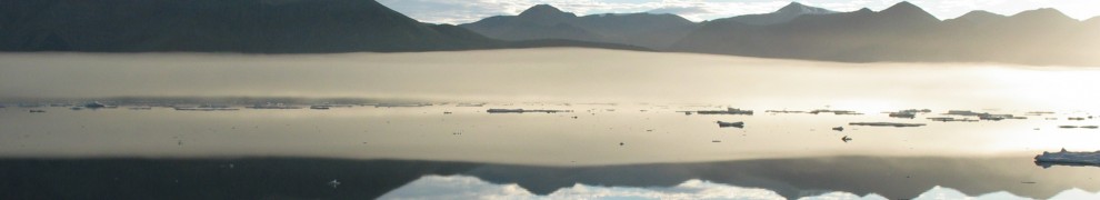
After four months of total darkness the sun is back up in Nares Strait. It transforms the polar night into thousand shades of white as mountains, glaciers, and ice take in and throw back the new light. Our satellites receive some of the throw-away light as the landscape reflects it back into space. During the long dark winter months these satellites could only “see” heat, but this will change rapidly as Alert atop of Arctic Canada receives 30 minutes more sun with each passing day.
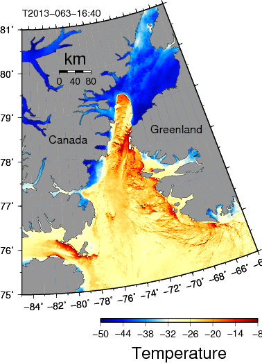
Surface temperature in degrees centigrade over northern Baffin Bay on March-4, 2013 16:20 UTC from MODIS Terra. Warm colors (reds) show thin and/or ice while cold colors (blues) suggest thick ice stuck in place.
A very strong ice arch at the southern entrance to Nares Strait separates thick (and cold) ice to north from thin (and warm) ice to the south. The thick and cold ice is not moving, it is stuck to land, but the ocean under the ice is moving fast from north to south. The ocean currents thus sweep the newly formed thin ice away to the south. This ice arch formed way back in early November just after the sun set for winter over Nares Strait.
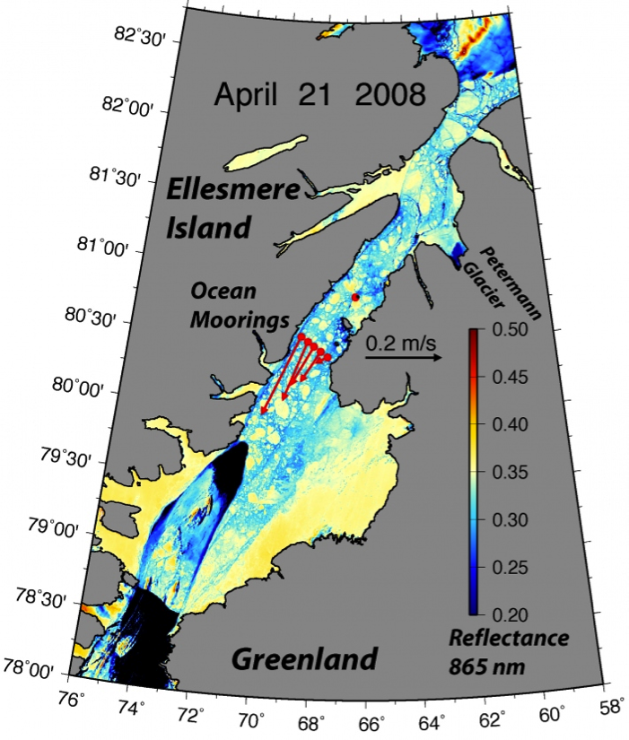
Now that the sun is up, we can also “see” more structures in the ice by the amount of light reflected back to space. A very white surface reflects lots while a darker surface reflects less. We are looking at the many shades of white here … even though I color them in reds and blues:

Surface reflectance at 865 nm in northern Baffin Bay on March-4, 2013 16:20 UTC from MODIS Terra. A true color image (which this is not) would show only white everywhere. Hence I show the very bright white as red and the less bright white as blue. This artificial enhancement makes patterns and structures more visible to the eye.
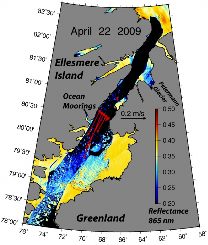
Zooming into the area where the ice arch separates thick ice to the north that is not moving from thin ice in the south that is swept away by ocean currents, I show this image at the highest possible resolution:

Surface reflectance at 865 nm at the southern entrance to Nares Strait on March-4, 2013. Contours are 200-m bottom depth showing PII2012 grounded at the north-eastern sector of the ice arch.
Note, however, that the sun is far to south and barely peeking over the horizon. This low sun angle shows up as shadows cast by mountains. And since the sun is still far to the south, the shadows cast are to the north. This “shadow” makes visible the ice island from Petermann Gletscher that anchors this ice arch as it is grounded. I labeled it PII2012 in the picture.
From laser measurements we know that the ice islands stands about 20 meter (or 60 feet) above the rest of the ice field. This height is enough to cast a visible shadow towards the north (slightly darker = less red) as well as a direct reflection off its vertical wall facing south (brighter = more red) towards the sun. At its thickest point, PII2012 is about 200 meters (~600 feet) thick. For this reason, I also show the 200-m bottom contour that moves largely from north to south along both Ellesmere Island, Canada on the left and Greenland on the right.
The sun brings great joy to all, especially those hardy souls who live in the far north. The sun’s rise also shows the delicate interplay of light and shadows that we can use to solve puzzles on how ice, oceans, and glaciers work. At the entrance of Nares Strait the playful delights of the sea ice, ocean currents, and ice islands gives us a large area of thin ice. The thin ice will soon melt and perhaps has already started to set into motion a spring bloom of ocean plants. Ocean critters will feed on these to start another cycle of life. Whales, seals, and polar bears all depend on it for 1000s of years now.
![Sketch of the biological pieces that a large area of open water near a fixed ice edge like that of a polynya may support. [From Northern Journal>/a>]](https://icyseas.org/wp-content/uploads/2013/03/polynya.jpg)
Sketch of the biological pieces that a large area of open water near a fixed ice edge like that of a polynya may support. [From Northern Journal]
![Polar Bear seen Oct.-10, 2003 from aboard the USCGS Healy to the north-east of Alaska [Credit: Andreas Muenchow, University of Delawarel]](https://icyseas.org/wp-content/uploads/2013/02/healy2003polarbear.jpg)
![Polar bear as seen in Kennedy Channel on Aug.-12, 2012. [Photo Credit: Kirk McNeil, Labrador from aboard the Canadian Coast Guard Ship Henry Larsen]](https://icyseas.org/wp-content/uploads/2012/08/polarbear-kirkmcneil_0418.jpg)
![Polar bear population and their trends. [Source: Polar Bear Specialist Group. Laris Karklis/The Washington Post. Published on December 23, 2012, 5:24 p.m.]](https://icyseas.org/wp-content/uploads/2013/02/w-polarbear24b.jpg)