While Viking rulers of Kyiv in Ukraine formally converted to Christianity in 988 CE at the outer limits of eastern Europe, two small viking settlements emerged at the southern tip of Greenland close to the Americas. The Norse settlers of Greenland left Iceland with 25 ships, but 11 of these either turned back to Iceland or were lost at sea. The remaining 14 boats arrived near 61 N latitude to establish an “Eastern” settlement which over time grew to more than 190 farms and 12 churches. Farther north near 64 N latitude a smaller “Western” settlement eventually grew to about 90 farms and four churches near Nuuk, today’s capital of Greenland. The “Western” settlement had a warmer and milder continental climate, because their farms were located far inland within a wide and complex fjord system that sheltered the farmers from atrocious coastal storms. The “Eastern” settlement was hit harder by these storms, because here the farms were closer to shore, closer to the icesheet, and closer to the center of the North-Atlantic storm activity.

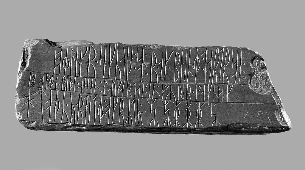
For about 200-300 years the settlements flourished and reached a population of about 4,000 people. They paid taxes to the King of Norway, donated tithes to their churches, and imported clothing, iron, and food stuff from Scandinavia. They paid with ivory from narwhales and walrus that they hunted in Disko Bay at 69 N latitude. Three viking hunters scratched their names in stone on a cairn they built about 1333 CE on an island near Upernavik at 73 N latitude (Francis, 2011). At these “Northern Hunting Grounds” the vikings from both “Eastern” and “Western” settlements likely met the Inuit of the Thule culture who at the time were moving south along West Greenland after a 3000 km migration from coastal Alaska within a few generations.
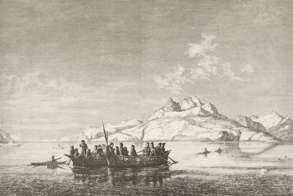
The modern Inuit of the Thule culture arrived in Greenland about 200-300 years after the vikings did. They arrived on foot, by dog sled, and in umiaks from the Bering Sea area of Alaska and Siberia (Friesen, 2016). They were equally adept to hunt caribou on land with bow and arrow, seals on sea ice with spears, and whales on open ocean with sophisticated harpoons. They crossed Smith Sound at 79 N latitude about 1300 CE to reach Greenland spreading south towards the viking settlements and north-east towards Fram Strait separating Greenland from Svalbard. On a beach off Independence Fjord in North-East Greenland at almost 83 N latitude Eigil Knuth found the frame of one of their skin-hulled umiak in 1949 (Knuth, 1952).
The vikings built “permanent” houses of stone, farmed the land, and kept sheep, goat, and cows. They hunted walrus and narwhal for its ivory to trade with Europe to import metals, clothes, and foods. Their diet until about 1300 CE was high on terrestrial and low on marine resources as indicated by isotopic studies of their bone structure. This changed when a cooling climate challenged animal husbandry in Greenland and the Norse transitioned towards a marine-based diet of fish, seals, and marine mamals (Jackson et al., 2018).
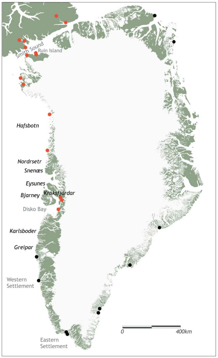
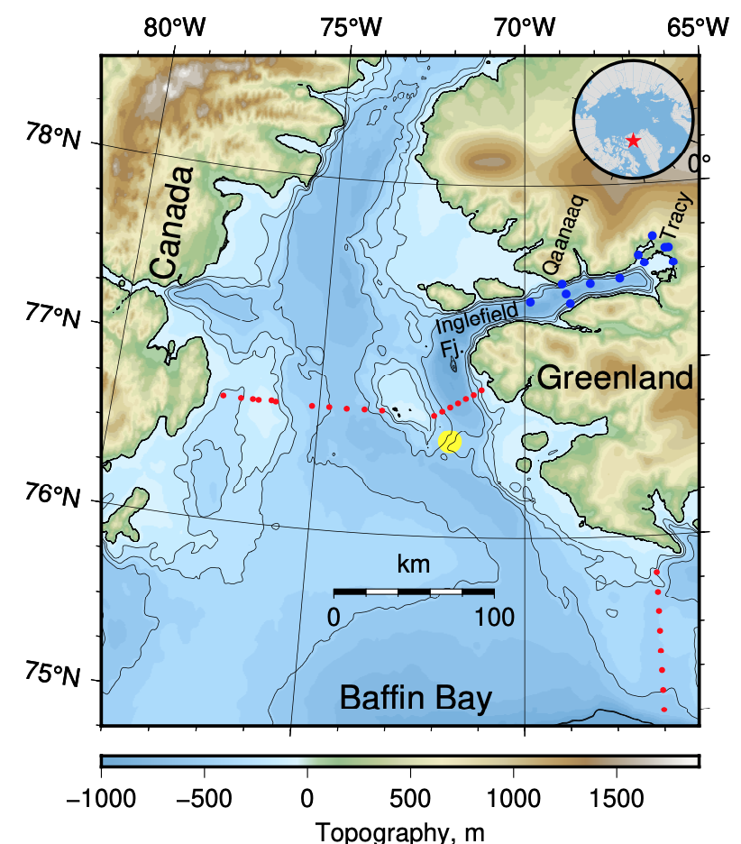
Map of Greenland and Ellesmere Islands adapted from Gullov (2008). Red symbols indicate Norse artifacts found at Inuit sites occupied in the 13th and 14th century while black dots represent location of such artifacts at 15th and 16th century.
In contrast, the Inuit embraced a more mobile life-style as entire family units moved large distances to new sites from year to year and seasonally from summer to winter camps. Their hunting was tied to the sea ice and they developed fancy techniques to hunt larger whales, walrus, and polar bears for food, fuel, and clothing. Their technologies and behaviors adapted rapidly in an extreme environment and climate that kept changing in time. Inuit often viewed themselves and their animal prey as mutually connected with energies flowing from animal to Inuit and vice versa. Both were part of one nature which changes in time on many different cycles that one needs to read and understand for survival. This view differed from that of the more pastoral vikings who saw themselves and their homes as “safe inner spaces” and everything on the outside as “wild and hostile” nature. They constantly tried to modify, improve, and control the landscape while the Inuit moved and adapted within it (Jackson et al., 2018).
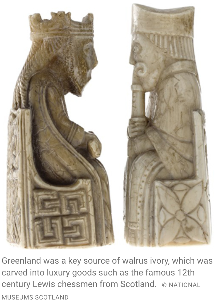
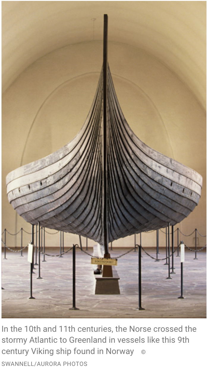
Viking settlement on Greenland (left), chess figures from walrus ivory (center), and viking longboat from the 10th century.
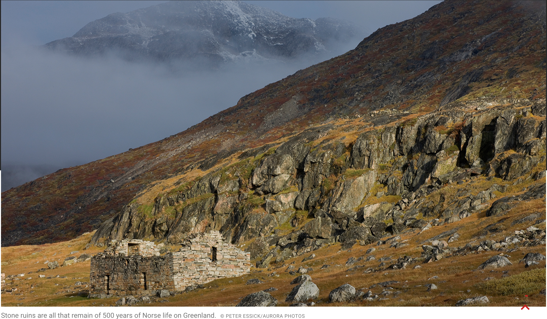
The vikings vanished without a trace in the 15th century. Their fate is still researched and debated in academic and popular outlets alike. In contrast, the Inuit expanded their range along all of Greenland where in the 18th and 19th centuries they were “re-discovered” in the South by Danish and Moravian colonists and missionaries and in the North by the English Navy, American adventurers, and Danish scientists.
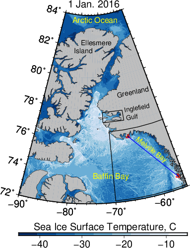
In 1910 two Danes Knut Rasmussen and Peter Freuchen established a trading post at North Star Bay near 77 N Latitude. They called “Thule.” Over the next 20 years Thule became a focal point of about 200 nomadic Inughuit that all are direct descendants of the Thule culture Inuit. There are about 700 of them today and most still live in Qaanaaq. Linguist Stephen Pax Leonard lived among them for a year in 2010/11 when he produced a 10 minute video that documents contemporary Inuit life and language.

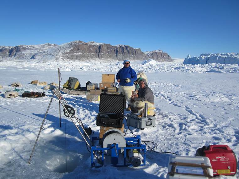
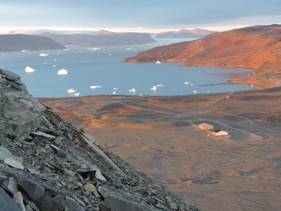
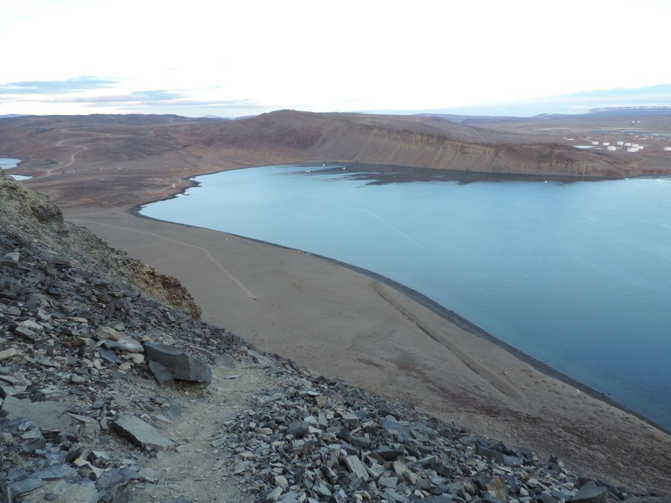
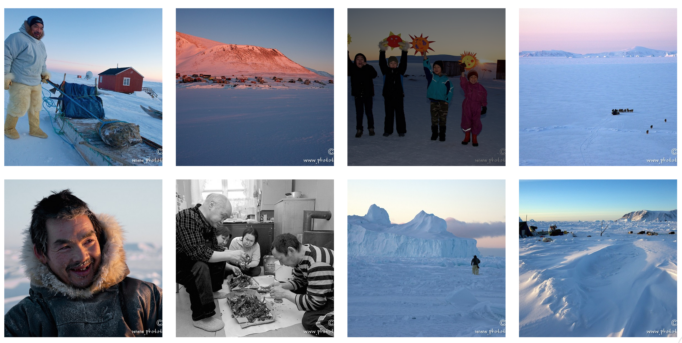
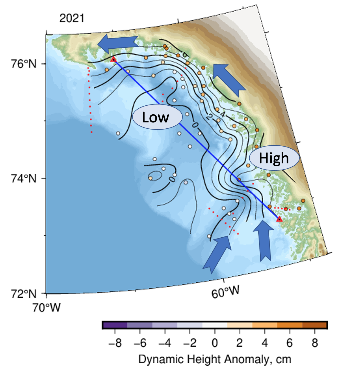
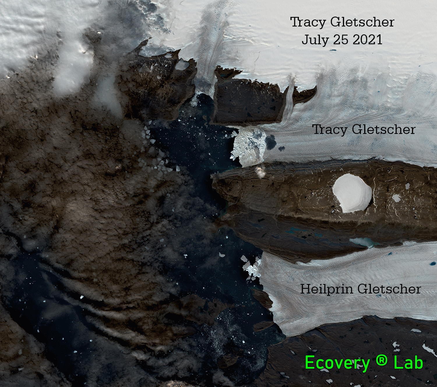
Contemporary photos of Qaanaaq and Thule region. Photos on left panel by Dr. Steffen Olsen near Tracy Glacier in Inglefield Fjord while images in right panel are of North Star Bay and Thule Air Base by the author.
References:
Francis, C.S., 2011: The Lost Western Settlements of Greenland, 1342, California State Univ. Sacramento, MA Thesis, 84 pp.
Friesen, T.M., 2016: Pan-Arctic Population Movements, Chap.-28 of “The Prehistoric Arctic,” Oxford Univ. Press, 988 pp.
Gullov, H.C., 2008: The Nature of Contact between Native Greenlanders and Norse, J. North Atlantic, 1, 16-24.
Jackson, R., J. Arneborg, A. Dugmore, C. Madsen, T. McGovern, K. Smiarowski, R. Streeter, 2018: Disequilibrium, Adaptation, and the Norse Settlement of Greenland, Human Ecology, 46 (5), https://doi.org/10.1007/s10745-018-0020-0.
Kintsch, E., 2016: Why did Greenland’s Vikings disappear? Science, 10.1126/science.aal0363, accessed as https://www.science.org/content/article/why-did-greenland-s-vikings-disappear
Knuth, E., 1952: An Outline of the Archaeology of Peary Land, Arctic, 5(1), pp. 17-33.